1 Introduction

From the 2000’s we had to study a new concept in management sciences. It was ‘Business Intelligence’ (BI). Krauth (2008) summarized the actual information about Business Intelligence and also forecasted the expected development and changes of BI for the next ten years. One of the priorities changes he emphasized was that ‘Technologies providing business intelligence will leave the corporate framework and move on a much wider scale to serve the growing demands of organizations and individuals for accurate, substantial and comprehensible information.’

After ten years we saw that the demand was actually raised in the leaders of small and medium enterprises also for the dissolution of business intelligence, furthermore there are several so-called self-service business intelligence solutions we should use to satisfy this demand. From the 2010s we could see that the basic technology of business informatics the online analytical processing (OLAP) was released in scientific research also, mainly in processing measured data.

In the 2000s business environment – mainly in small and medium enterprises – unfortunately we saw that neither the economists nor the IT staff of these small firms could work with this BI-solutions (softwares). The reason for the problem is not in technical difficulties but in acquiring the right way of thinking to model the function of their own firm, define correctly the information requirement of management (conceptual modeling) and translate it to a logical model.

We participated in a data warehouse projects where we realized that our ‘corporate bus matrix’ contained about 80–120 indicators with nearly 200 dimensions (dimensional attributes), therefore we started to work on the early stenography to formalize the management question (Takács & Bubnó 2012).

2 Related Works

It is an often-mentioned problem today in the literature that there is no standardized or widely agreed method for implementing the conceptual model (Bánné 2012; Macedo & Oliviera 2015; Rizzi 2008). Furthermore, it is a good practice to try to follow the classical design steps of database systems (Halassy 1994) in the design of the data warehouse (conceptual model->logical model->physical model->implementation), but opinions differ in the literature which should be the right order of the steps, furthermore, there is a lot of overlap. Mainly conceptual and logical modeling are often mixed with each other or their borders are blurred, however Halassy clearly defined the levels of database planning, furthermore he proved that these levels must be separated from each other (Halassy 1994).

According to the method presented by us, the conceptual model is nothing more than a set of formalized leadership questions. A management question can already be seen as part of an OLAP data cube, and OLAP cubes can be built from subsets of management questions. The question is to optimize their number and distribution. That is, how many cubes do we have to build and how many questions can be answered. While the former is a matter of financial concern for customers, the latter is about the efficiency of the information system.

As regards data warehouses as information systems, the question of efficiency is most of all the above-mentioned two aspects (cost and amount of information that can be extracted). Di Tria, Lefons, & Tangorra (2017) tested design methodologies and carried out for cost-effectiveness analysis. They have set up their framework and metrics to implement this analysis. The classic approaches of data warehouse design can be sorted into two sets: data driven methods and requirement driven methods. Both have advantages and limitations also (Di Tria, Lefons, & Tangorra 2017). For example, the requirement driven approach leads such multidimensional schemas that usually results in one data cube that answer only one question of the management. The main problem with the multidimensional schemas of the other approach is the big number of the potential questions which cause data lakes that become data swamps. We consider a cuboid as a base of a potential management question. The problem is: what is the minimal (optimal cost) number of cuboids? These problems with both approaches lead to the birth of several so-called hybrid modeling methods to design data warehouses. Di Tria, Lefons, & Tangorra (2017) identified the criteria based on the literature to evaluate these hybrid methods. They used the 4 common and main criteria that is necessary to evaluate a data warehouse designing methodology. These are: Correctness, Completeness, Minimality and Understandability (Halassy 1994). Furthermore, based on the literature they defined metrics to the evaluation of costs and benefits, specially the ‘Metrics for schema quality’ and the ‘Metrics for design effort’. Then they compare six hybrid methods based on this framework:

1. Graph-based Hybrid Multidimensional model (referred to as GrHyMM),
2. UML for Data Warehouse (referred to as UMLDW),
3. Multidimensional Design by Example (referred to as MDBE),
4. Phipps&Davis Methodology (referred to as PDM),
5. Goal-oriented Requirement Analysis for Data Warehouse Design (referred to as GRAnD),
6. Goal/Question/Metric-based Methodology (referred to as GQM).

Based on Di Tria, Lefons, & Tangorra (2017) in Table 1 we present the steps of the six methodologies above and the features or results of the certain steps, extended with our Visualized Management Question-based Design methodology (referred to as VMQD*).

Our Visualized Management Question-based Design methodology is closest to GQM in the steps, but there are some differences.

1. Requirement Analysis. We collect questions with metrics and dimensionality of the problem also in this phase with the required visualizations from the decision makers via interviews. Then we formalize these specifications with our special structured stenography that is based on the terminology corresponding to the current problem. The output of this step is a set of formalized questions.
2. Deriving minimal granularity. Based on the set of formalized questions we specify the required minimal granularity for every indicator. The output of this step is the set of indicators with minimally detailed dimensions.
3. Deriving ideal schemata. We map the dimensional attributes and values to keys, produce the initial conceptual schemata. The output of this step contains ideal dimensions (keys, attributes and hierarchies) and ideal facts (with dimension keys for join), independently from the sources.
4. Source Analysis. The main question of this step is: What kind of transactions can we get them from? We decompose ideal facts into potential elementary transactional attributes and identify them in the source systems. The output of this step is the derived potential schemata.
5. Integration. Ideal schemata from the requirement analysis are compared with potential star schemata. Match occurs, when the two schemata contain the same fact, and, both have the same dimensionality in the same granularity level. In this step we define required transformations and calculate fact tables and common dimensions with attributes.
6. Multidimensional modeling. We build the cube(s) with dimensions, dimension hierarchies and measures.

We used the Di Tria, Lefons, & Tangorra (2017) notation to visualize the framework of our methodology for better comparison (Figure 1).

Every question of the management is a visualization of aggregated indicator(s) detailed with dimensional attribute(s). So, we must formalize these questions of the management.

The formalisation has to cover:

• aggregations (aggregate functions)
  i.e. sum, min, max, average, count, median, modus, correlation, etc.;
• indicators with unit
  i.e. Price^$, Quantity^pcs, Weight^kg, etc.;
• visualization
  i.e. table, line chart, map, network graphs, population pyramid, etc.;
• attributes
  i.e. Gender, Product name, City, Order date, etc.;
• attribute aggregation
  i.e. sum, min, max, average, rate, distribution, etc.;
• dimensions
  i.e. Person, Product, Geography, Date, etc.;
• dimension hierarchies
  i.e. Product->Product category, City->County->Country->Continent

The structure and syntax of the formalization is:

3 Methodology of formalization of conceptual design

In the following paragraph we would like to explain our methodology.

1. In the phase of requirement analysis, we collect and formalize management questions. The question and description are defined in a textual and formal way. The ‘manager’ is the person for whom the system provides information. As a result, she expects to see a data-visualization report appearing on different dashboards. The reports and dashboards need to be configured according to the requirements of access rights (what kind of level managers can access the statements).
   In the requirement analysis, we ‘analyse’ the management question based on the following considerations in Table 2:
   What is the indicator? In which aggregation? What is the unit? Which visualization we want to see? in Which detail(s)? Is there a slicer?
   Formally: $I_{\left\{\text{af}\left[,\text{af}\right]\right\}}^{\left\{u\left[,u\right]\right\}}{\left(\begin{array}{c}\mathrm{vt}\\ \left[\left\{\begin{array}{c}s\\ s\end{array}\right\}\right]\end{array}\right)}^v\left[{\left(\begin{array}{c}{D}_{{{\displaystyle \sum }}^{}\left\{a\right\}}\\ \left[D_{{{\displaystyle \sum }}^{}\left\{a\right\}}\right]\end{array}\right)}^{\left\{d\right\}}\right]$M2 \documentclass[10pt]{article} \usepackage{wasysym} \usepackage[substack]{amsmath} \usepackage{amsfonts} \usepackage{amssymb} \usepackage{amsbsy} \usepackage[mathscr]{eucal} \usepackage{mathrsfs} \usepackage{pmc} \usepackage[Euler]{upgreek} \pagestyle{empty} \oddsidemargin -1.0in \begin{document} \[ {\boldsymbol{I}}_{\left\{ {{\rm{af}}\left[ {,{\rm{af}}} \right]} \right\}}^{\left\{ {u\left[ {,u} \right]} \right\}}{\left({\begin{array}{*{20}{c}} {vt}\\ {\left[ {\left\{ {\begin{array}{*{20}{c}} s\\ s \end{array}} \right\}} \right]} \end{array}} \right)^v}\left[ {{{\left({\begin{array}{*{20}{c}} {{{\boldsymbol{D}}_{\mathop \sum \nolimits^ \left\{ a \right\}}}}\\ {\left[ {{{\boldsymbol{D}}_{\mathop \sum \nolimits^ \left\{ a \right\}}}} \right]} \end{array}} \right)}^{\{ d\} }}} \right] \] \end{document}
   This formal definition is related to one diagram. Several different visualizations need to arise from the leader on a question related to the requirement specification, so many formal descriptions are made in this section.
2. Deriving the minimum granularity for each indicator. Determine the indicators in the management question and determine the required minimum granularity (dimension and key), where:
   
   • I^{u} the indicator I with u unit(s) in the upper right index
   • D_{dk} dimension D with dimension key dk in the lower right index
   Formally: $I^{\left\{u\left[,u\right]\right\}}\left(D_{\left\{\mathrm{dk}\right\}}\left[,D_{\left\{\mathrm{dk}\right\}}\right]\right)$M3 \documentclass[10pt]{article} \usepackage{wasysym} \usepackage[substack]{amsmath} \usepackage{amsfonts} \usepackage{amssymb} \usepackage{amsbsy} \usepackage[mathscr]{eucal} \usepackage{mathrsfs} \usepackage{pmc} \usepackage[Euler]{upgreek} \pagestyle{empty} \oddsidemargin -1.0in \begin{document} \[ {{\boldsymbol{I}}^{\left\{ {u\left[ {,u} \right]} \right\}}}\left({{{\boldsymbol{D}}_{\left\{ {dk} \right\}}}\left[ {,{{\boldsymbol{D}}_{\left\{ {dk} \right\}}}} \right]} \right) \] \end{document}
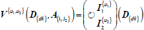
3. When we derive an ideal schemata, we produce fact tables for the indicators specified in the minimum granularity and optimizing the number of fact sheets. The properties are grouped into dimensions and hierarchies. Each dimension must have a dimension key (see relational data model), where:
   
   • I^{u} the indicator I with u unit(s) in the upper right index
   • D_{dk} dimension D with dimension key dk in the lower right index
   • D_{a} dimension D with attribute a in the lower right index
   • D_{i} dimension D with indicator i in the lower right index
   • D_{dhk} dimension D with dimension hierarchy key dhk in the lower right index, when hierarchy levels are stored in separate tables
   Fact tables formally: $I^{\left\{u\right\}}\left(D_{\left\{\mathrm{dk}\right\}}\left[,D_{\left\{\mathrm{dk}\right\}}\right]\right)$M4 \documentclass[10pt]{article} \usepackage{wasysym} \usepackage[substack]{amsmath} \usepackage{amsfonts} \usepackage{amssymb} \usepackage{amsbsy} \usepackage[mathscr]{eucal} \usepackage{mathrsfs} \usepackage{pmc} \usepackage[Euler]{upgreek} \pagestyle{empty} \oddsidemargin -1.0in \begin{document} \[ {{\boldsymbol{I}}^{\left\{ u \right\}}}\left({{{\boldsymbol{D}}_{\left\{ {dk} \right\}}}\left[ {,{{\boldsymbol{D}}_{\left\{ {dk} \right\}}}} \right]} \right) \] \end{document} , or $\left(\begin{array}{c}{I}^{\left\{u\right\}}\\ \left[I^{\left\{u\right\}}\right]\end{array}\right)\left(D_{\left\{\mathrm{dk}\right\}}\left[,D_{\left\{\mathrm{dk}\right\}}\right]\right)$M5 \documentclass[10pt]{article} \usepackage{wasysym} \usepackage[substack]{amsmath} \usepackage{amsfonts} \usepackage{amssymb} \usepackage{amsbsy} \usepackage[mathscr]{eucal} \usepackage{mathrsfs} \usepackage{pmc} \usepackage[Euler]{upgreek} \pagestyle{empty} \oddsidemargin -1.0in \begin{document} \[ \left({\begin{array}{*{20}{c}} {{{\boldsymbol{I}}^{\left\{ u \right\}}}}\\ {\left[ {{{\boldsymbol{I}}^{\left\{ u \right\}}}} \right]} \end{array}} \right)\left({{{\boldsymbol{D}}_{\left\{ {dk} \right\}}}\left[ {,{{\boldsymbol{D}}_{\left\{ {dk} \right\}}}} \right]} \right) \] \end{document} depending on whether the given fact table contains one or more indicators.
   Dimension table formally: $D\left(D_{\left\{\mathrm{dk}\right\}}\left[,D_{\left\{a\right\}}\right]\left[,D_{\left\{i\right\}}\right]\left[,D_{\left\{\mathrm{dhk}\right\}}\right]\right)$M6 \documentclass[10pt]{article} \usepackage{wasysym} \usepackage[substack]{amsmath} \usepackage{amsfonts} \usepackage{amssymb} \usepackage{amsbsy} \usepackage[mathscr]{eucal} \usepackage{mathrsfs} \usepackage{pmc} \usepackage[Euler]{upgreek} \pagestyle{empty} \oddsidemargin -1.0in \begin{document} \[ {\boldsymbol{D}}\left({{{\boldsymbol{D}}_{\left\{ {dk} \right\}}}\left[ {,{{\boldsymbol{D}}_{\left\{ a \right\}}}} \right]\left[ {,{{\boldsymbol{D}}_{\left\{ i \right\}}}} \right]\left[ {,{{\boldsymbol{D}}_{\left\{ {dhk} \right\}}}} \right]} \right) \] \end{document}
   During optimization we can notice one of the following cases in Table 3:
   • Different indicators with the same dimensionality and granularity can be grouped into one fact table.
   • Different indicators could be similar when they have the same dimensionality but diverging granularity, so we examine whether they can be produced from one another.
   • Dimensionality of one indicator is a proper subset of the dimensionality of the other indicator, so the other indicator dimensionality will be the minimum required.
4. We will evaluate the available data during the source analysis. Source system can be transaction-oriented or analysis-oriented.
   • The Transaction-Oriented Source System (OLTP) is characterized by a relational data model
     $E\left(E_{\left\{\mathrm{pk}\right\}}\left[,E_{\left\{a\right\}}\right]\left[,E_{\left\{\mathrm{fk}\right\}}\right]\right)$M7 \documentclass[10pt]{article} \usepackage{wasysym} \usepackage[substack]{amsmath} \usepackage{amsfonts} \usepackage{amssymb} \usepackage{amsbsy} \usepackage[mathscr]{eucal} \usepackage{mathrsfs} \usepackage{pmc} \usepackage[Euler]{upgreek} \pagestyle{empty} \oddsidemargin -1.0in \begin{document} \[ {\boldsymbol{E}}\left({{{\boldsymbol{E}}_{\left\{ {pk} \right\}}}\left[ {,{{\boldsymbol{E}}_{\left\{ a \right\}}}} \right]\left[ {,{{\boldsymbol{E}}_{\left\{ {fk} \right\}}}} \right]} \right) \] \end{document} and $R\left(E_{\left\{\mathrm{pk}\right\}}\left[,E_{\left\{\mathrm{pk}\right\}}\right],R_{\left\{a\right\}}\left[,R_{\left\{a\right\}}\right]\right)$M8 \documentclass[10pt]{article} \usepackage{wasysym} \usepackage[substack]{amsmath} \usepackage{amsfonts} \usepackage{amssymb} \usepackage{amsbsy} \usepackage[mathscr]{eucal} \usepackage{mathrsfs} \usepackage{pmc} \usepackage[Euler]{upgreek} \pagestyle{empty} \oddsidemargin -1.0in \begin{document} \[ {\boldsymbol{R}}\left({{{\boldsymbol{E}}_{\left\{ {pk} \right\}}}\left[ {,{{\boldsymbol{E}}_{\left\{ {pk} \right\}}}} \right],{{\boldsymbol{R}}_{\left\{ a \right\}}}\left[ {,{{\boldsymbol{R}}_{\left\{ a \right\}}}} \right]} \right) \] \end{document}
     where:
     • E( ) E entity in the source system,
     • E_{pk}pk primary key of E entity
     • E_{a}a attribute of E entity
     • E_{fk}fk foreign key of E entity
     • R( ) R relation, transaction between different entities, with the relational attributes
     • R_{a}a attribute of R relation
   • In the case of an Analysis-Oriented Source System (OLAP), the multidimensional relational model is typical.
     Fact tables formally: $I^{\left\{u\right\}}\left(D_{\left\{\mathrm{dk}\right\}}\left[,D_{\left\{\mathrm{dk}\right\}}\right]\right)$M9 \documentclass[10pt]{article} \usepackage{wasysym} \usepackage[substack]{amsmath} \usepackage{amsfonts} \usepackage{amssymb} \usepackage{amsbsy} \usepackage[mathscr]{eucal} \usepackage{mathrsfs} \usepackage{pmc} \usepackage[Euler]{upgreek} \pagestyle{empty} \oddsidemargin -1.0in \begin{document} \[ {{\boldsymbol{I}}^{\left\{ u \right\}}}\left({{{\boldsymbol{D}}_{\left\{ {dk} \right\}}}\left[ {,{{\boldsymbol{D}}_{\left\{ {dk} \right\}}}} \right]} \right) \] \end{document} , or $\left(\begin{array}{c}{I}^{\left\{u\right\}}\\ \left[I^{\left\{u\right\}}\right]\end{array}\right)\left(D_{\left\{\mathrm{dk}\right\}}\left[,D_{\left\{\mathrm{dk}\right\}}\right]\right)$M10 \documentclass[10pt]{article} \usepackage{wasysym} \usepackage[substack]{amsmath} \usepackage{amsfonts} \usepackage{amssymb} \usepackage{amsbsy} \usepackage[mathscr]{eucal} \usepackage{mathrsfs} \usepackage{pmc} \usepackage[Euler]{upgreek} \pagestyle{empty} \oddsidemargin -1.0in \begin{document} \[ \left({\begin{array}{*{20}{c}} {{{\boldsymbol{I}}^{\left\{ u \right\}}}}\\ {\left[ {{{\boldsymbol{I}}^{\left\{ u \right\}}}} \right]} \end{array}} \right)\left({{{\boldsymbol{D}}_{\left\{ {dk} \right\}}}\left[ {,{{\boldsymbol{D}}_{\left\{ {dk} \right\}}}} \right]} \right) \] \end{document} depending on whether the given fact table contains one or more indicators.
     Dimension table formally: $D\left(D_{\left\{\mathrm{dk}\right\}}\left[,D_{\left\{a\right\}}\right]\left[,D_{\left\{i\right\}}\right]\left[,D_{\left\{\mathrm{dhk}\right\}}\right]\right)$M11 \documentclass[10pt]{article} \usepackage{wasysym} \usepackage[substack]{amsmath} \usepackage{amsfonts} \usepackage{amssymb} \usepackage{amsbsy} \usepackage[mathscr]{eucal} \usepackage{mathrsfs} \usepackage{pmc} \usepackage[Euler]{upgreek} \pagestyle{empty} \oddsidemargin -1.0in \begin{document} \[ {\boldsymbol{D}}\left({{{\boldsymbol{D}}_{\left\{ {dk} \right\}}}\left[ {,{{\boldsymbol{D}}_{\left\{ a \right\}}}} \right]\left[ {,{{\boldsymbol{D}}_{\left\{ i \right\}}}} \right]\left[ {,{{\boldsymbol{D}}_{\left\{ {dhk} \right\}}}} \right]} \right) \] \end{document} , wehere:
     • I^{u} the indicator I with u unit(s) in the upper right index
     • D_{dk} dimension D with dimension key dk in the lower right index
     • D_{a} dimension D with attribute a in the lower right index
     • D_{i} dimension D with indicator i in the lower right index
     • D_{dhk} dimension D with dimension hierarchy key dhk in the lower right index, when hierarchy levels are stored in separate tables
5. During integration, we coordinate the ideal data model with the available source system data. Describe the requirements that include attributes, dimension keys, and additional indicators to use. We design the data loading (ETL/ELT) process in Table 4.

Table 3

Optimizations’ notations.

$\left(\begin{array}{c}{I}_1\\ I_2\end{array}\right)\left(D_{\left\{\mathrm{dk}\right\}}\right)\equiv I_1\left(D_{\left\{\mathrm{dk}\right\}}\right)\times I_2\left(D_{\left\{\mathrm{dk}\right\}}\right)$M16 \documentclass[10pt]{article} \usepackage{wasysym} \usepackage[substack]{amsmath} \usepackage{amsfonts} \usepackage{amssymb} \usepackage{amsbsy} \usepackage[mathscr]{eucal} \usepackage{mathrsfs} \usepackage{pmc} \usepackage[Euler]{upgreek} \pagestyle{empty} \oddsidemargin -1.0in \begin{document} \[ \left({\begin{array}{*{20}{c}} {{{\boldsymbol{I}}_1}}\\ {{{\boldsymbol{I}}_2}} \end{array}} \right)\left({{{\boldsymbol{D}}_{\left\{ {dk} \right\}}}} \right) \equiv {{\boldsymbol{I}}_1}\left({{{\boldsymbol{D}}_{\left\{ {dk} \right\}}}} \right) \times {{\boldsymbol{I}}_2}\left({{{\boldsymbol{D}}_{\left\{ {dk} \right\}}}} \right) \] \end{document}	Combining indicators I1 and I2 with the same dimensionality. We create the Descartes multiplier of the two indicators.
	The value of the indicator I can be obtained by summing through dimension D (roll up) with the aggregate function in the lower left index of I. Calculating the aggregation from D{dk} at the bottom of the Summa symbol to the level at the top of the Summa sign (all or D{dhk} hierarchy level, leaving the original key. This is referred to as .
$\begin{array}{l}{I}_1\left(A_{\left\{\mathrm{dk}\right\}}\right)\subset I_2\left(A_{\left\{\mathrm{dk}\right\}},B_{\left\{\mathrm{dk}\right\}}\right)\\ \left(\begin{array}{c}{I}_1\left(A_{\left\{\mathrm{dk}\right\}}\right)\\ I_2\left(A_{\left\{\mathrm{dk}\right\}},B_{\left\{\mathrm{dk}\right\}}\right)\end{array}\right)\equiv \left(\begin{array}{c}{I}_1\\ I_2\end{array}\right)\left(A_{\left\{\mathrm{dk}\right\}},B_{\left\{\mathrm{dk}\right\}}\right)\end{array}$M19 \documentclass[10pt]{article} \usepackage{wasysym} \usepackage[substack]{amsmath} \usepackage{amsfonts} \usepackage{amssymb} \usepackage{amsbsy} \usepackage[mathscr]{eucal} \usepackage{mathrsfs} \usepackage{pmc} \usepackage[Euler]{upgreek} \pagestyle{empty} \oddsidemargin -1.0in \begin{document} \[ \begin{array}{l} {{\boldsymbol{I}}_1}\left({{{\boldsymbol{A}}_{\left\{ {dk} \right\}}}} \right) \subset {{\boldsymbol{I}}_2}\left({{{\boldsymbol{A}}_{\left\{ {dk} \right\}}},{{\boldsymbol{B}}_{\left\{ {dk} \right\}}}} \right)\\ \left({\begin{array}{*{20}{c}} {{{\boldsymbol{I}}_1}\left({{{\boldsymbol{A}}_{\left\{ {dk} \right\}}}} \right)}\\ {{{\boldsymbol{I}}_2}\left({{{\boldsymbol{A}}_{\left\{ {dk} \right\}}},{{\boldsymbol{B}}_{\left\{ {dk} \right\}}}} \right)} \end{array}} \right) \equiv \left({\begin{array}{*{20}{c}} {{{\boldsymbol{I}}_1}}\\ {{{\boldsymbol{I}}_2}} \end{array}} \right)\left({{{\boldsymbol{A}}_{\left\{ {dk} \right\}}},{{\boldsymbol{B}}_{\left\{ {dk} \right\}}}} \right) \end{array} \] \end{document}	A and B are dimensions of indicators I1 and I2 and I1 is proper subset of I2.

Table 4

Data loadings’ transformation notations.

	The value of the indicator I can be obtained by summing through D dimension (roll up) with the aggregate function in the lower left index of I. This is an aggregation is from D{dk} at the bottom of the Summa symbol to the level at the top of the Summa Sign (all or D{dhk} hierarchy level, leaving the original key. This is referred to as .
$D\left(D_{\left\{\mathrm{dk}\right\}}\left[,D_{\left\{a\right\}}\right]\left[,D_{\left\{i\right\}}\right]\right)=D\left({\displaystyle \sum _{D_{\left\{\mathrm{dk}\right\}}}^{D_{\left\{\mathrm{dk}\right\}}}}\left[,D_{\left\{a\right\}}\right]\left[,{}_{\text{af}}{}^{}D{}_{\left\{i\right\}}\right]\right)$M22 \documentclass[10pt]{article} \usepackage{wasysym} \usepackage[substack]{amsmath} \usepackage{amsfonts} \usepackage{amssymb} \usepackage{amsbsy} \usepackage[mathscr]{eucal} \usepackage{mathrsfs} \usepackage{pmc} \usepackage[Euler]{upgreek} \pagestyle{empty} \oddsidemargin -1.0in \begin{document} \[ {\boldsymbol{D}}\left({{{\boldsymbol{D}}_{\left\{ {dk} \right\}}}\left[ {,{{\boldsymbol{D}}_{\left\{ a \right\}}}} \right]\left[ {,{{\boldsymbol{D}}_{\left\{ i \right\}}}} \right]} \right) = {\boldsymbol{D}}\left({\sum\limits_{{{\boldsymbol{D}}_{\left\{ {dk} \right\}}}}^{{{\boldsymbol{D}}_{\left\{ {dk} \right\}}}} {} \left[ {,{{\boldsymbol{D}}_{\left\{ a \right\}}}} \right]\left[ {,{}_{{\rm{af}}}^{}{{\boldsymbol{D}}_{\left\{ i \right\}}}} \right]} \right) \] \end{document}	Deduplicate the values of D dimensions’ D{dk}. key. Summarize the indicator with the af aggregate function in the lower left index, while leaving the first element of attribute values.
$I\left(D_{\left\{\mathrm{dk}\right\}}\right)=I\left(\right)\times D_{\left\{\mathrm{dk}\right\}}$M23 \documentclass[10pt]{article} \usepackage{wasysym} \usepackage[substack]{amsmath} \usepackage{amsfonts} \usepackage{amssymb} \usepackage{amsbsy} \usepackage[mathscr]{eucal} \usepackage{mathrsfs} \usepackage{pmc} \usepackage[Euler]{upgreek} \pagestyle{empty} \oddsidemargin -1.0in \begin{document} \[ {\boldsymbol{I}}\left({{{\boldsymbol{D}}_{\left\{ {dk} \right\}}}} \right) = {\boldsymbol{I}}\left({} \right) \times {{\boldsymbol{D}}_{\left\{ {dk} \right\}}} \] \end{document}	Expand the dimensionality of indicator I. The Descartes multiplier of the original indicator with the dimension to be expanded.
	Pivoting I indicator values through D{a} dimensional attribute. We create several new indicators corresponding to the occurrence values of the attribute.
$\left(\begin{array}{c}{I}_1\\ I_2\end{array}\right)\left(D_{\left\{\mathrm{dk}\right\}}\right)=I_1\left(D_{\left\{\mathrm{dk}\right\}}\right)\times I_2\left(D_{\left\{\mathrm{dk}\right\}}\right)$M25 \documentclass[10pt]{article} \usepackage{wasysym} \usepackage[substack]{amsmath} \usepackage{amsfonts} \usepackage{amssymb} \usepackage{amsbsy} \usepackage[mathscr]{eucal} \usepackage{mathrsfs} \usepackage{pmc} \usepackage[Euler]{upgreek} \pagestyle{empty} \oddsidemargin -1.0in \begin{document} \[ \left({\begin{array}{*{20}{c}} {{{\boldsymbol{I}}_1}}\\ {{{\boldsymbol{I}}_2}} \end{array}} \right)\left({{{\boldsymbol{D}}_{\left\{ {dk} \right\}}}} \right) = {{\boldsymbol{I}}_1}\left({{{\boldsymbol{D}}_{\left\{ {dk} \right\}}}} \right) \times {{\boldsymbol{I}}_2}\left({{{\boldsymbol{D}}_{\left\{ {dk} \right\}}}} \right) \] \end{document}	Combining I1 I2 indicators with the same dimensionality. We create the Descartes multiplier of the two indicators.
	Unpivoting I1 I2 indicators with the same dimensionality into V indicator values and A attribute set with the indicators’ name
$I={\displaystyle \sum }_{D_{\left\{a\right\}}}^{\mathrm{all}}{I}_{D_{\left\{a\right\}}}$M27 \documentclass[10pt]{article} \usepackage{wasysym} \usepackage[substack]{amsmath} \usepackage{amsfonts} \usepackage{amssymb} \usepackage{amsbsy} \usepackage[mathscr]{eucal} \usepackage{mathrsfs} \usepackage{pmc} \usepackage[Euler]{upgreek} \pagestyle{empty} \oddsidemargin -1.0in \begin{document} \[ {\boldsymbol{I}} = \mathop \sum \limits_{{{\boldsymbol{D}}_{\left\{ a \right\}}}}^{all} {{\boldsymbol{I}}_{{{\boldsymbol{D}}_{\left\{ a \right\}}}}} \] \end{document}	The sum of pivoted $I_{D_{\left\{a\right\}}}$M28 \documentclass[10pt]{article} \usepackage{wasysym} \usepackage[substack]{amsmath} \usepackage{amsfonts} \usepackage{amssymb} \usepackage{amsbsy} \usepackage[mathscr]{eucal} \usepackage{mathrsfs} \usepackage{pmc} \usepackage[Euler]{upgreek} \pagestyle{empty} \oddsidemargin -1.0in \begin{document} \[ {{\boldsymbol{I}}_{{{\boldsymbol{D}}_{\left\{ a \right\}}}}} \] \end{document} indicator values along the occurrence values of D{a} attribute.

In the data loading process, extracting, transforming, and loading only those keys, attributes, and indicators from the source system to the data warehouse that we need.

During the transformation of data, two types of data loading processes can be discussed:

• During ETL (Extract, Transform, Load) process the various data manipulations carried out after extracting the data from the source system are typically in an intermediate system (Staging Area) and then transferred to the data warehouse. Intermediate use of complex multi-step data manipulations (transform) is needed, for simpler systems it is worth thinking about using it as it can serve more data warehouses with intermediate data than a commonly used general date dimension, geographical dimension, organizational dimension (enterprise data lake).

The transformations can be simple, then the indicators are loaded from one source system relation, and the dimensions are also derived from a single source system.

The transformations may be more complicated when the values of the indicators are loaded from several relations’ attributes or from several different source systems. This also occurs with the indicators of dimension.

• During ELT (Extract, Load, Transform) process the various data manipulations take place after the data is extracted from the source system and loaded into the data warehouse.
  When we formalize a business question, the method is pure requirement-driven. We do not bother with data-driven approach at this stage. We bother with it after we have collected and formalized and modelled all the questions, and the required data model is generated, then we examine the questions through the data-driven approach also. At this point we examine how the formalized elements of the questions are stored in the source systems. If we can produce them in the required granularity (or more detailed) then we optimize them (for example with the use of some kind of aggregation function) to the ETL/ELT (Extract-Transform-Load/Extract-Load-Transform) processes.

4 Research data processing example (Collecting and processing fitness tracker data)

The relationship between physical inactivity and some chronic health conditions is a widely researched area but further efforts are needed to assist people to adopt healthier lifestyles (Lee et al. 2012). Using wearable activity trackers can be a promising opportunity for individuals to improve lifestyle behaviour (Maher et al. 2017). There are several studies in this area, mainly from the lifestyle behaviour and health approach (Henriksen et al. 2018; Kaewkannate & Kim 2016; Karapanos et al. 2016). Our research does not examine activity trackers from the aspect of health, we want to present the way that we can process data with OLAP technology we collected with a very simple device. If an end user who wants to know his own activity by using such an activity tracker, usually he downloads a software that processes his data every day and informs him. But if we plan a wide research where we want to collect several persons’ data, and we want to recognize trends and patterns in the behaviour of the society, it could be a useful approach if we plan a data cube with OLAP approach. With our hybrid design methodology, we get metadata from the dimensions and attributes, so if we extract our data into a dataset, we get the formal description of the structure of our dataset also, in order to share and compare it to other similar researches.

Our research investigated the physical activity of university students using fitness tracker. Participants in the pilot test had to meet several criteria. Participants had to wear the device with normal living conditions for 90 consecutive days, which simulated the normal living conditions of most students. An important element of the long-term pilot test is that it can represent the full range of normal people’s activities in a real environment. Each participant was informed on the most important information about the device and the potential for managing possible sources of error. The battery of the bracelet was recharged by the users every 20 days, depending on the use, whereby the data was collected at the same time. The data was sent by the users for one week on a daily basis and then at the charges mentioned above. This level of data supply has served to reduce the potential loss of data. We informed the students about the study and all the participants provided informed consent in compliance with the principles of the Declaration of Helsinki (WMA 2013) and the new GDPR (EP 2016). The study was approved by the Regional Ethics Board (DE RKEB/IKEB: 4843-2017) at the Clinical Canter of the University of Debrecen.

Collected bracelets’ data are processed using OLAP technology. We use the following hybrid design methodology and formal descriptive techniques to design, implement, and document the operations related to the information system (Research Data Warehouse) that we produce.

4.3 Ideal schemata for OLAP system

In this step we determine which indicators can be stored in a common fact table.

During optimization, we can see which indicators are similar and can be produced from one another. In this case activity indicator detailed by GenderKey (GK) can be generated from the activity indicator detailed by PersonKey (PK). This means that we have already managed to optimize the number of indicators we are building.

$\mathrm{Activit}{y}_{}^{\left\{\mathrm{day}\right\}}\left(P_{\left\{\mathrm{GK}\right\}},D_{\left\{\mathrm{MK}\right\}},I_{\left\{\mathrm{IK}\right\}}\right)\equiv \mathrm{Activit}{y}_{}^{\left\{\mathrm{day}\right\}}\left({\displaystyle \sum _{P_{\left\{\mathrm{pk}\right\}}}^{P_{\left\{\mathrm{GK}\right\}}}},D_{\left\{\mathrm{MK}\right\}},I_{\left\{\mathrm{IK}\right\}}\right)$

M63 \documentclass[10pt]{article} \usepackage{wasysym} \usepackage[substack]{amsmath} \usepackage{amsfonts} \usepackage{amssymb} \usepackage{amsbsy} \usepackage[mathscr]{eucal} \usepackage{mathrsfs} \usepackage{pmc} \usepackage[Euler]{upgreek} \pagestyle{empty} \oddsidemargin -1.0in \begin{document} \[ {\boldsymbol{Activity}}_{}^{\left\{ {day} \right\}}\left({{{\boldsymbol{P}}_{\left\{ {GK} \right\}}},{{\boldsymbol{D}}_{\left\{ {MK} \right\}}},{{\boldsymbol{I}}_{\left\{ {IK} \right\}}}} \right) \equiv {\boldsymbol{Activity}}_{}^{\left\{ {day} \right\}}\left({\sum\limits_{{{\boldsymbol{P}}_{\left\{ {PK} \right\}}}}^{{{\boldsymbol{P}}_{\left\{ {GK} \right\}}}} {}, {{\boldsymbol{D}}_{\left\{ {MK} \right\}}},{{\boldsymbol{I}}_{\left\{ {IK} \right\}}}} \right) \] \end{document}

$\mathrm{Activit}{y}_{}^{\left\{\mathrm{day}\right\}}\left({\displaystyle \sum _{P_{\left\{\mathrm{pk}\right\}}}^{P_{\left\{\mathrm{GK}\right\}}}},D_{\left\{\mathrm{MK}\right\}},I_{\left\{\mathrm{IK}\right\}}\right)\stackrel{\min }{\Leftarrow }\mathrm{Activit}{y}_{}^{\left\{\mathrm{day}\right\}}\left(P_{\left\{\mathrm{pk}\right\}},D_{\left\{\mathrm{MK}\right\}},I_{\left\{\mathrm{IK}\right\}}\right)$

M64 \documentclass[10pt]{article} \usepackage{wasysym} \usepackage[substack]{amsmath} \usepackage{amsfonts} \usepackage{amssymb} \usepackage{amsbsy} \usepackage[mathscr]{eucal} \usepackage{mathrsfs} \usepackage{pmc} \usepackage[Euler]{upgreek} \pagestyle{empty} \oddsidemargin -1.0in \begin{document} \[ {\boldsymbol{Activity}}_{}^{\left\{ {day} \right\}}\left({\sum\limits_{{{\boldsymbol{P}}_{\left\{ {PK} \right\}}}}^{{{\boldsymbol{P}}_{\left\{ {GK} \right\}}}} {}, {{\boldsymbol{D}}_{\left\{ {MK} \right\}}},{{\boldsymbol{I}}_{\left\{ {IK} \right\}}}} \right)\mathop \Leftarrow \limits^{min} {\boldsymbol{Activity}}_{}^{\left\{ {day} \right\}}\left({{{\boldsymbol{P}}_{\left\{ {PK} \right\}}},{{\boldsymbol{D}}_{\left\{ {MK} \right\}}},{{\boldsymbol{I}}_{\left\{ {IK} \right\}}}} \right) \] \end{document}

The average DailySteps indicator must break down into gender variants and the aggregated.

$\mathrm{DailyStep}{s}_{\text{average}}^{\left\{\mathrm{steps}\right\}}\left({\displaystyle \sum _{P_{\left\{\mathrm{GK}\right\}}}^{\mathrm{all}}},D_{\left\{\mathrm{dk}\right\}}\right)\equiv \mathrm{AverageDailyStep}{s}_{}^{\left\{\mathrm{steps}\right\}}\left(D_{\left\{\mathrm{dk}\right\}}\right)$

M65 \documentclass[10pt]{article} \usepackage{wasysym} \usepackage[substack]{amsmath} \usepackage{amsfonts} \usepackage{amssymb} \usepackage{amsbsy} \usepackage[mathscr]{eucal} \usepackage{mathrsfs} \usepackage{pmc} \usepackage[Euler]{upgreek} \pagestyle{empty} \oddsidemargin -1.0in \begin{document} \[ {\boldsymbol{DailySteps}}_{{\rm{average}}}^{\left\{ {steps} \right\}}\left({\sum\limits_{{{\boldsymbol{P}}_{\left\{ {GK} \right\}}}}^{all} {}, {{\boldsymbol{D}}_{\left\{ {DK} \right\}}}} \right) \equiv {\boldsymbol{AverageDailySteps}}_{}^{\left\{ {steps} \right\}}\left({{{\boldsymbol{D}}_{\left\{ {DK} \right\}}}} \right) \] \end{document}

Next step is to place indicators into fact tables. Indicators with the same dimensionality and granularity are placed into a common fact table. In this case these are the daily activity and the daily steps fact tables.

ftDailyActivity: Daily activity fact table

$\mathrm{Activit}{y}_{}^{\left\{\mathrm{day}\right\}}\left(P_{\left\{\mathrm{pk}\right\}},D_{\left\{\mathrm{MK}\right\}},I_{\left\{\mathrm{IK}\right\}}\right)$

M68 \documentclass[10pt]{article} \usepackage{wasysym} \usepackage[substack]{amsmath} \usepackage{amsfonts} \usepackage{amssymb} \usepackage{amsbsy} \usepackage[mathscr]{eucal} \usepackage{mathrsfs} \usepackage{pmc} \usepackage[Euler]{upgreek} \pagestyle{empty} \oddsidemargin -1.0in \begin{document} \[ {\boldsymbol{Activity}}_{}^{\left\{ {day} \right\}}\left({{{\boldsymbol{P}}_{\left\{ {PK} \right\}}},{{\boldsymbol{D}}_{\left\{ {MK} \right\}}},{{\boldsymbol{I}}_{\left\{ {IK} \right\}}}} \right) \] \end{document}

ftDailySteps: Daily steps fact table

$\left(\begin{array}{c}\mathrm{AverageDailyStep}{s}_{}^{\left\{\mathrm{steps}\right\}}\\ \mathrm{AverageDailyStep}{s}_{\text{Male}}^{\left\{\mathrm{steps}\right\}}\\ \mathrm{AverageDailyStep}{s}_{\text{Female}}^{\left\{\mathrm{steps}\right\}}\end{array}\right)\left(D_{\left\{\mathrm{dk}\right\}}\right)\equiv \mathrm{AverageDailyStep}{s}_{P_{{{\displaystyle \sum }}^{}\left\{\mathrm{gender}\right\}}}^{\left\{\mathrm{steps}\right\}}\left(D_{\left\{\mathrm{dk}\right\}}\right)$

M69 \documentclass[10pt]{article} \usepackage{wasysym} \usepackage[substack]{amsmath} \usepackage{amsfonts} \usepackage{amssymb} \usepackage{amsbsy} \usepackage[mathscr]{eucal} \usepackage{mathrsfs} \usepackage{pmc} \usepackage[Euler]{upgreek} \pagestyle{empty} \oddsidemargin -1.0in \begin{document} \[ \left({\begin{array}{*{20}{c}} {{\boldsymbol{AverageDailySteps}}_{}^{\left\{ {steps} \right\}}}\\ {{\boldsymbol{AverageDailySteps}}_{{\rm{Male}}}^{\left\{ {steps} \right\}}}\\ {{\boldsymbol{AverageDailySteps}}_{{\rm{Female}}}^{\left\{ {steps} \right\}}} \end{array}} \right)\left({{{\boldsymbol{D}}_{\left\{ {DK} \right\}}}} \right) \equiv {\boldsymbol{AverageDailySteps}}_{{{\boldsymbol{P}}_{\mathop \sum \nolimits^ \left\{ {gender} \right\}}}}^{\left\{ {steps} \right\}}\left({{{\boldsymbol{D}}_{\left\{ {DK} \right\}}}} \right) \] \end{document}

Dimensional attributes and values in questions and dimensional keys in the minimal and ideal data model must be organized into dimensions. In this step we specify the Dimension->Key-Attribute-Indicator->Value structures, also the required dimension hierarchies with hierarchy-keys. We have three dimensions (Person, Date, Intensity) in our ideal data model in the following structure:

• P: Person (dimPerson)
  • PersonKey (P_{PK}): HASH of students’ identifier
  • Student (P_{stud}): students’ identifier (eliminated, because of GDPR)
  • GenderKey (P_{GK}): unique identifier, values {1, 2} (eliminated, when we unfold the dimension hierarchy)
  • Gender (P_{gender}): gender of students, values {Male, Female}
• D: Date (dimDate)
  • DateKey (D_{DK}): year, month, day serial number with leading zero, composition {yyyy}{mm}{dd}
  • Day of Week (D_{DoW}): unique identifier, serial number of weekdays {1..7} (eliminated, when we partly unfold the dimension hierarchy)
  • Weekday (D_{weekday}): {1 – Monday, 2 – Tuesday, …, 7 – Sunday}
  • MonthKey (D_{MK}): year, month serial number with leading zero, composition {yyyy}{mm}
  • DM: DateMonth (dimDateMonth)
    • MonthKey (DM_{MK}): year, month serial number with leading zero, composition {yyyy}{mm}
    • Month (DM_{month}): month name, values {January, February, …, December}
• I: Intensity (dimIntensity): Categories of daily activity of students.
  • IntensityKey (I_{IK}): {0..5}
  • Daily Step Category (I_{dsc}):
    • 0 – Basal activity
    • 1 – Limited activity
    • 2 – Low activity
    • 3 – Somewhat active
    • 4 – Active
    • 5 – Highly active

4.4 Source analysis

In this phase we discover the data of the source systems driven by the facts and dimensions specified in the ideal data model.

4.4.1 Activity tracker data

S_iOS (S_{steps}, S_{timestamp}, S_{date}, S_{10min},) Emails sent via email from iPhone, the name of the file contains the student’s Neptun identifier and the date of submission in the S_{NID}–S_{sd} structure.

S_A (S_{{cumulative steps}}, S_{timestamp}, S_{date}, S_{min},) Emails sent via email from Android phone, the name of the file contains the student’s Neptun identifier and the date of submission in the S_{NID}–S_{sd} structure.

• S: Steps (noted as rSteps) with the following attributes and values:
  • Date (S_{date}): {year}.{month}.{day}
  • DateKey (S_{DK}): {year}{month}{day}
  • 10mins (S_{10mins}): {hh}:{m0}:{00}
  • minute (S_{min}): {hh}:{mm}:{00}
  • TimeKey (S_{TK}): S_{10min} mapping to [0..143] integers closed interval
  • timestamp (S_{timestamp}): in seconds, the number of seconds passed since 1900.01.00 0:00:00
  • StepSum_iOS (S_{steps}): number of steps taken in 10 minutes
  • StepSum_A (S_{{cumulative steps}}): the number of daily steps taken to a given time
  • StepType (S_{st}): {raw, normalized}
  • 10minNS (S_{10mNS}): 10-minute normalized step data
  • Neptun identifier (S_{NID}): the NEPTUN identifier of the student submitting the data
  • Person key (S_{PK}): the hashed NEPTUN identifier of the student submitting the data
  • Submission date (S_{sd}): date of data submission in {year}{month}{day} structure
  • ETL date (S_{etld}): the date key of the ETL process in {year}{month}{day} structure
  • From ‘source systems’ the data is loaded into an intermediate storage.
  • We supplement each standalone file with the data in its name and the step type dependent on the mobile operating system.

$S_{\mathrm{iOS}}\left(S_{\left\{\mathrm{steps}\right\}},S_{\left\{\mathrm{timestamp}\right\}},S_{\left\{\mathrm{date}\right\}},S_{\left\{10\min \right\}}\right)\times (S_{\left\{\mathrm{NID}\right\}},S_{\left\{\mathrm{sd}\right\}},S_{\left\{\mathrm{etld}\right\}})\times S_{\left\{\text{normalized}\right\}}$

M70 \documentclass[10pt]{article} \usepackage{wasysym} \usepackage[substack]{amsmath} \usepackage{amsfonts} \usepackage{amssymb} \usepackage{amsbsy} \usepackage[mathscr]{eucal} \usepackage{mathrsfs} \usepackage{pmc} \usepackage[Euler]{upgreek} \pagestyle{empty} \oddsidemargin -1.0in \begin{document} \[ {{\boldsymbol{S}}_{iOS}}\left({{{\boldsymbol{S}}_{\left\{ {steps} \right\}}},{{\boldsymbol{S}}_{\left\{ {timestamp} \right\}}},{{\boldsymbol{S}}_{\left\{ {date} \right\}}},{{\boldsymbol{S}}_{\left\{ {10min} \right\}}}} \right) \times ({{\boldsymbol{S}}_{\left\{ {NID} \right\}}},{{\boldsymbol{S}}_{\left\{ {sd} \right\}}},{{\boldsymbol{S}}_{\left\{ {etld} \right\}}}) \times {{\boldsymbol{S}}_{\left\{ {{\rm{normalized}}} \right\}}} \] \end{document}

 

$S_A\left(S_{\left\{\mathrm{cumulative} \hspace{0.17em}\mathrm{steps}\right\}},S_{\left\{\mathrm{timestamp}\right\}},S_{\left\{\mathrm{date}\right\}},S_{\left\{\min \right\}}\right)\times (S_{\left\{\mathrm{NID}\right\}},S_{\left\{\mathrm{sd}\right\}},S_{\left\{\mathrm{etld}\right\}})\times S_{\left\{\text{raw}\right\}}$

M71 \documentclass[10pt]{article} \usepackage{wasysym} \usepackage[substack]{amsmath} \usepackage{amsfonts} \usepackage{amssymb} \usepackage{amsbsy} \usepackage[mathscr]{eucal} \usepackage{mathrsfs} \usepackage{pmc} \usepackage[Euler]{upgreek} \pagestyle{empty} \oddsidemargin -1.0in \begin{document} \[ {{\boldsymbol{S}}_A}\left({{{\boldsymbol{S}}_{\left\{ {cumulative\,steps} \right\}}},{{\boldsymbol{S}}_{\left\{ {timestamp} \right\}}},{{\boldsymbol{S}}_{\left\{ {date} \right\}}},{{\boldsymbol{S}}_{\left\{ {min} \right\}}}} \right) \times ({{\boldsymbol{S}}_{\left\{ {NID} \right\}}},{{\boldsymbol{S}}_{\left\{ {sd} \right\}}},{{\boldsymbol{S}}_{\left\{ {etld} \right\}}}) \times {{\boldsymbol{S}}_{\left\{ {{\rm{raw}}} \right\}}} \] \end{document}

The data from the Android phone (S_{{cumulative steps}}) is a cumulative step number for a given time, so we must first calculate its dynamics (increment for the previous measurement).

$\begin{array}{l}\hspace{0.17em}\hspace{0.17em}\hspace{0.17em}\hspace{0.17em}\hspace{0.17em}\hspace{0.17em}\hspace{0.17em}\hspace{0.17em}\hspace{0.17em}\hspace{0.17em}\hspace{0.17em}\hspace{0.17em}\hspace{0.17em}\hspace{0.17em}\hspace{0.17em}\hspace{0.17em}\hspace{0.17em}\hspace{0.17em}\hspace{0.17em}\hspace{0.17em}\hspace{0.17em}\hspace{0.17em}\hspace{0.17em}\hspace{0.17em}\hspace{0.17em}\hspace{0.17em}\hspace{0.17em}\hspace{0.17em}\hspace{0.17em}\hspace{0.17em}\hspace{0.17em}\hspace{0.17em}\hspace{0.17em}\hspace{0.17em}\hspace{0.17em}\hspace{0.17em}\hspace{0.17em}\hspace{0.17em}\hspace{0.17em}\hspace{0.17em}\hspace{0.17em}\hspace{0.17em}\hspace{0.17em}\hspace{0.17em}\hspace{0.17em}\hspace{0.17em}\hspace{0.17em}\hspace{0.17em}\hspace{0.17em}\hspace{0.17em}\hspace{0.17em}\hspace{0.17em}\hspace{0.17em}\hspace{0.17em}\hspace{0.17em}\hspace{0.17em}\hspace{0.17em}\hspace{0.17em}\hspace{0.17em}\hspace{0.17em}\hspace{0.17em}\hspace{0.17em}\hspace{0.17em}\hspace{0.17em}\hspace{0.17em}\hspace{0.17em}\hspace{0.17em}\hspace{0.17em}\hspace{0.17em}\hspace{0.17em}\hspace{0.17em}\hspace{0.17em}\hspace{0.17em}\hspace{0.17em}\hspace{0.17em}{S}_A\left(S_{\left\{\mathrm{steps}\right\}},S_{\left\{\mathrm{timestamp}\right\}},S_{\left\{\mathrm{date}\right\}},S_{\left\{\min \right\}},S_{\left\{\mathrm{NID}\right\}},S_{\left\{\mathrm{sd}\right\}},S_{\left\{\mathrm{etld}\right\}},S_{\left\{\text{raw}\right\}}\right) \\ \hspace{0.17em}\hspace{0.17em}\hspace{0.17em}\hspace{0.17em}\hspace{0.17em}\hspace{0.17em}\hspace{0.17em}\hspace{0.17em}\hspace{0.17em}\hspace{0.17em}\hspace{0.17em}\hspace{0.17em}\hspace{0.17em}\hspace{0.17em}\hspace{0.17em}\hspace{0.17em}\hspace{0.17em}\hspace{0.17em}\hspace{0.17em}\hspace{0.17em}\hspace{0.17em}\hspace{0.17em}\hspace{0.17em}\hspace{0.17em}\hspace{0.17em}\hspace{0.17em}\hspace{0.17em}\hspace{0.17em}\hspace{0.17em}\hspace{0.17em}\hspace{0.17em}\hspace{0.17em}\hspace{0.17em}\hspace{0.17em}\hspace{0.17em}\hspace{0.17em}\hspace{0.17em}\hspace{0.17em}\hspace{0.17em}\hspace{0.17em}\hspace{0.17em}\hspace{0.17em}\hspace{0.17em}\hspace{0.17em}\hspace{0.17em}\hspace{0.17em}\hspace{0.17em}\hspace{0.17em}\hspace{0.17em}\hspace{0.17em}\hspace{0.17em}\hspace{0.17em}\hspace{0.17em}\hspace{0.17em}\hspace{0.17em}\hspace{0.17em}\hspace{0.17em}\hspace{0.17em}\hspace{0.17em}\hspace{0.17em}\hspace{0.17em}\hspace{0.17em}\hspace{0.17em}\hspace{0.17em}\hspace{0.17em}\hspace{0.17em}\hspace{0.17em}\hspace{0.17em}\hspace{0.17em}\hspace{0.17em}\hspace{0.17em}\hspace{0.17em}\hspace{0.17em}\hspace{0.17em}\hspace{0.17em}\hspace{0.17em}\hspace{0.17em}\hspace{0.17em}\hspace{0.17em}\hspace{0.17em}\hspace{0.17em}\hspace{0.17em}\hspace{0.17em}\hspace{0.17em}\hspace{0.17em}\hspace{0.17em}\hspace{0.17em}\hspace{0.17em}\hspace{0.17em}\hspace{0.17em}\hspace{0.17em}\hspace{0.17em}\hspace{0.17em}\hspace{0.17em}\hspace{0.17em}\hspace{0.17em}\hspace{0.17em}\hspace{0.17em}\hspace{0.17em}\hspace{0.17em}\hspace{0.17em}\hspace{0.17em}\hspace{0.17em}\hspace{0.17em}\hspace{0.17em}\hspace{0.17em}\hspace{0.17em}\hspace{0.17em}\hspace{0.17em}\hspace{0.17em}\hspace{0.17em}\hspace{0.17em}\hspace{0.17em}\hspace{0.17em}\hspace{0.17em}\hspace{0.17em}\hspace{0.17em}\hspace{0.17em}\hspace{0.17em}\hspace{0.17em}\hspace{0.17em}\hspace{0.17em}\hspace{0.17em}\hspace{0.17em}\hspace{0.17em}\hspace{0.17em}\hspace{0.17em}\hspace{0.17em}\hspace{0.17em}\hspace{0.17em}\hspace{0.17em}\hspace{0.17em}\hspace{0.17em}\hspace{0.17em}\hspace{0.17em}\hspace{0.17em}\hspace{0.17em}\hspace{0.17em}\hspace{0.17em}\hspace{0.17em}\hspace{0.17em}\hspace{0.17em}\hspace{0.17em}\hspace{0.17em}\hspace{0.17em}\hspace{0.17em}\hspace{0.17em}\hspace{0.17em}\hspace{0.17em}\hspace{0.17em}\hspace{0.17em}\hspace{0.17em}=\\ \underset{i=1}{\overset{n}{{\displaystyle \cup }}}\left(S_A^i\left(S_{\left\{\mathrm{cumulative} \mathrm{steps}\right\}}\right)-\{\begin{array}{c}0, \mathrm{if} \neg \exists L_A^{i-1}\vee \left(S_A^{i-1}\left(L_{\left\{\mathrm{date}\right\}}\right)\ne S_A^i\left(S_{\left\{\mathrm{date}\right\}}\right)\right)\vee \left(S_A^{i-1}\left(S_{\left\{\mathrm{NID}\right\}}\right)\ne S_A^i\left(S_{\left\{\mathrm{NID}\right\}}\right)\right)\\ S_A^{i-1}\left(S_{\left\{\mathrm{cumulative} \mathrm{steps}\right\}}\right), \mathrm{if} \exists S_A^{i-1}\wedge \left(S_A^{i-1}\left(S_{\left\{\mathrm{date}\right\}}\right)=S_A^i\left(S_{\left\{\mathrm{date}\right\}}\right)\right)\wedge \left(S_A^{i-1}\left(S_{\left\{\mathrm{NID}\right\}}\right)=S_A^i\left(S_{\left\{\mathrm{NID}\right\}}\right)\right)\end{array}\right)\\ \hspace{0.17em}\hspace{0.17em}\hspace{0.17em}\hspace{0.17em}\hspace{0.17em}\hspace{0.17em}\hspace{0.17em}\hspace{0.17em}\hspace{0.17em}\hspace{0.17em}\hspace{0.17em}\hspace{0.17em}\hspace{0.17em}\hspace{0.17em}\hspace{0.17em}\hspace{0.17em}\hspace{0.17em}\hspace{0.17em}\hspace{0.17em}\hspace{0.17em}\hspace{0.17em}\hspace{0.17em}\hspace{0.17em}\hspace{0.17em}\hspace{0.17em}\hspace{0.17em}\hspace{0.17em}\hspace{0.17em}\hspace{0.17em}\hspace{0.17em}\hspace{0.17em}\hspace{0.17em}\hspace{0.17em}\hspace{0.17em}\hspace{0.17em}\hspace{0.17em}\hspace{0.17em}\hspace{0.17em}\hspace{0.17em}\hspace{0.17em}\hspace{0.17em}\hspace{0.17em}\hspace{0.17em}\hspace{0.17em}\hspace{0.17em}\hspace{0.17em}\hspace{0.17em}\hspace{0.17em}\hspace{0.17em}\hspace{0.17em}\hspace{0.17em}\hspace{0.17em}\hspace{0.17em}\hspace{0.17em}\hspace{0.17em}\hspace{0.17em}\hspace{0.17em}\hspace{0.17em}\hspace{0.17em}\hspace{0.17em}\times \left(S_{\left\{\mathrm{timestamp}\right\}},S_{\left\{\mathrm{date}\right\}},S_{\left\{\min \right\}},S_{\left\{\mathrm{NID}\right\}},S_{\left\{\mathrm{sd}\right\}},S_{\left\{\mathrm{etld}\right\}},S_{\left\{\text{raw}\right\}}\right)\end{array}$

M72 \documentclass[10pt]{article} \usepackage{wasysym} \usepackage[substack]{amsmath} \usepackage{amsfonts} \usepackage{amssymb} \usepackage{amsbsy} \usepackage[mathscr]{eucal} \usepackage{mathrsfs} \usepackage{pmc} \usepackage[Euler]{upgreek} \pagestyle{empty} \oddsidemargin -1.0in \begin{document} \[ \begin{array}{l} \quad\qquad\qquad\qquad\qquad{{\boldsymbol{S}}_A}\left({{{\boldsymbol{S}}_{\left\{ {steps} \right\}}},{{\boldsymbol{S}}_{\left\{ {timestamp} \right\}}},{{\boldsymbol{S}}_{\left\{ {date} \right\}}},{{\boldsymbol{S}}_{\left\{ {min} \right\}}},{{\boldsymbol{S}}_{\left\{ {NID} \right\}}},{{\boldsymbol{S}}_{\left\{ {sd} \right\}}},{{\boldsymbol{S}}_{\left\{ {etld} \right\}}},{{\boldsymbol{S}}_{\left\{ {{\rm{raw}}} \right\}}}} \right){\rm{}}\\ \qquad\qquad\qquad\qquad\qquad\qquad\qquad\qquad\qquad\qquad\, = \\ \mathop \cup \limits_{i = 1}^n \left({{\boldsymbol{S}}_A^i\left({{{\boldsymbol{S}}_{\left\{ {cumulative\quad steps} \right\}}}} \right) - \left\{ {\begin{array}{*{20}{c}} {0,\ if{\rm{}}\neg \exists {\boldsymbol{L}}_A^{i - 1} \vee \left({{\boldsymbol{S}}_A^{i - 1}\left({{{\boldsymbol{L}}_{\left\{ {date} \right\}}}} \right) \ne {\boldsymbol{S}}_A^i\left({{{\boldsymbol{S}}_{\left\{ {date} \right\}}}} \right)} \right) \vee \left({{\boldsymbol{S}}_A^{i - 1}\left({{{\boldsymbol{S}}_{\left\{ {NID} \right\}}}} \right) \ne {\boldsymbol{S}}_A^i\left({{{\boldsymbol{S}}_{\left\{ {NID} \right\}}}} \right)} \right)}\\ {{\boldsymbol{S}}_A^{i - 1}\left({{{\boldsymbol{S}}_{\left\{ {cumulative\quad steps} \right\}}}} \right),\quad if\quad \exists {\boldsymbol{S}}_A^{i - 1} \wedge \left({{\boldsymbol{S}}_A^{i - 1}\left({{{\boldsymbol{S}}_{\left\{ {date} \right\}}}} \right) = {\boldsymbol{S}}_A^i\left({{{\boldsymbol{S}}_{\left\{ {date} \right\}}}} \right)} \right) \wedge \left({{\boldsymbol{S}}_A^{i - 1}\left({{{\boldsymbol{S}}_{\left\{ {NID} \right\}}}} \right) = {\boldsymbol{S}}_A^i\left({{{\boldsymbol{S}}_{\left\{ {NID} \right\}}}} \right)} \right)} \end{array}} \right.} \right)\\ \quad\qquad\qquad\qquad\qquad\, \times \left({{{\boldsymbol{S}}_{\left\{ {timestamp} \right\}}},{{\boldsymbol{S}}_{\left\{ {date} \right\}}},{{\boldsymbol{S}}_{\left\{ {min} \right\}}},{{\boldsymbol{S}}_{\left\{ {NID} \right\}}},{{\boldsymbol{S}}_{\left\{ {sd} \right\}}},{{\boldsymbol{S}}_{\left\{ {etld} \right\}}},{{\boldsymbol{S}}_{\left\{ {{\rm{raw}}} \right\}}}} \right) \end{array} \] \end{document}

Finally, we generate a common large data source from many individual files:

$\begin{array}{c}{S}_A\left(S_{\left\{\mathrm{steps}\right\}},S_{\left\{\mathrm{timestamp}\right\}},S_{\left\{\mathrm{date}\right\}},S_{\left\{\min \right\}},\underset{S_{\left\{\mathrm{NID}\right\}}}{\overset{\mathrm{all}}{{\displaystyle \cup }}}{S}_{\mathrm{NID}},S_{\left\{\mathrm{sd}\right\}},S_{\left\{\mathrm{etld}\right\}},S_{\left\{\text{raw}\right\}}\right)\\ {{\displaystyle \cup }}^{}\\ S_{\mathrm{iOS}}\left(S_{\left\{\mathrm{steps}\right\}},S_{\left\{\mathrm{timestamp}\right\}},S_{\left\{\mathrm{date}\right\}},S_{\left\{10\min \right\}},\underset{S_{\left\{\mathrm{NID}\right\}}}{\overset{\mathrm{all}}{{\displaystyle \cup }}}{S}_{\left\{\mathrm{NID}\right\}},S_{\left\{\mathrm{sd}\right\}},S_{\left\{\mathrm{etld}\right\}},S_{\left\{\text{normalized}\right\}}\right)\end{array}$

M73 \documentclass[10pt]{article} \usepackage{wasysym} \usepackage[substack]{amsmath} \usepackage{amsfonts} \usepackage{amssymb} \usepackage{amsbsy} \usepackage[mathscr]{eucal} \usepackage{mathrsfs} \usepackage{pmc} \usepackage[Euler]{upgreek} \pagestyle{empty} \oddsidemargin -1.0in \begin{document} \[ \begin{array}{*{20}{c}} {{{\boldsymbol{S}}_A}\left({{{\boldsymbol{S}}_{\left\{ {steps} \right\}}},{{\boldsymbol{S}}_{\left\{ {timestamp} \right\}}},{{\boldsymbol{S}}_{\left\{ {date} \right\}}},{{\boldsymbol{S}}_{\left\{ {min} \right\}}},\mathop \cup \limits_{{{\boldsymbol{S}}_{\left\{ {NID} \right\}}}}^{all} {{\boldsymbol{S}}_{NID}},{{\boldsymbol{S}}_{\left\{ {sd} \right\}}},{{\boldsymbol{S}}_{\left\{ {etld} \right\}}},{{\boldsymbol{S}}_{\left\{ {{\rm{raw}}} \right\}}}} \right)}\\ \qquad\qquad\qquad{\mathop \cup \nolimits}\\ {{{\boldsymbol{S}}_{iOS}}\left({{{\boldsymbol{S}}_{\left\{ {steps} \right\}}},{{\boldsymbol{S}}_{\left\{ {timestamp} \right\}}},{{\boldsymbol{S}}_{\left\{ {date} \right\}}},{{\boldsymbol{S}}_{\left\{ {10min} \right\}}},\mathop \cup \limits_{{{\boldsymbol{S}}_{\left\{ {NID} \right\}}}}^{all} {{\boldsymbol{S}}_{\left\{ {NID} \right\}}},{{\boldsymbol{S}}_{\left\{ {sd} \right\}}},{{\boldsymbol{S}}_{\left\{ {etld} \right\}}},{{\boldsymbol{S}}_{\left\{ {{\rm{normalized}}} \right\}}}} \right)} \end{array}{\rm{}} \] \end{document}

We generate 10-minute time intervals data from the activity tracker data. Data from the android phone Time property with minute accuracy is 10 minutes raw data, must be normalized as 10-minute accuracy data. The timekey value $S_{\left\{\mathrm{tkv}\right\}}^i=\mathrm{Nr}(S_{\left\{\min \right\}})*144$M74 \documentclass[10pt]{article} \usepackage{wasysym} \usepackage[substack]{amsmath} \usepackage{amsfonts} \usepackage{amssymb} \usepackage{amsbsy} \usepackage[mathscr]{eucal} \usepackage{mathrsfs} \usepackage{pmc} \usepackage[Euler]{upgreek} \pagestyle{empty} \oddsidemargin -1.0in \begin{document} \[ {\boldsymbol{S}}_{\left\{ {tkv} \right\}}^i = Nr({{\boldsymbol{S}}_{\left\{ {min} \right\}}})*144 \] \end{document} will be a real number on the closed interval [0..144], the corresponding time key $S_{\left\{\mathrm{TK}\right\}}^i=\mathrm{int}(\mathrm{Nr}(S_{\left\{\min \right\}})*144)$M75 \documentclass[10pt]{article} \usepackage{wasysym} \usepackage[substack]{amsmath} \usepackage{amsfonts} \usepackage{amssymb} \usepackage{amsbsy} \usepackage[mathscr]{eucal} \usepackage{mathrsfs} \usepackage{pmc} \usepackage[Euler]{upgreek} \pagestyle{empty} \oddsidemargin -1.0in \begin{document} \[ {\boldsymbol{S}}_{\left\{ {TK} \right\}}^i = int(Nr({{\boldsymbol{S}}_{\left\{ {min} \right\}}})*144) \] \end{document} is the whole part of the real number.

Each S_{steps} value must be broken down into the current 10-minute increments and the previous 10-minute increments. This brings out normalized Android bracelet data.

$\begin{array}{c}\underset{i=1}{\overset{n}{{\displaystyle \cup }}}\hspace{0.17em}{S}_A^i\left(S_{\left\{\mathrm{steps}\right\}}\text{*}\left(S_{\left\{\mathrm{tkv}\right\}}^i-S_{\left\{\mathrm{TK}\right\}}^i\right)\right)\times \left(S_{\left\{\mathrm{timestamp}\right\}},S_{\left\{\mathrm{date}\right\}},S_{\left\{\mathrm{TK}\right\}},S_{\left\{\mathrm{NID}\right\}},S_{\left\{\mathrm{sd}\right\}},S_{\left\{\mathrm{etld}\right\}},S_{\left\{\text{normalized}\right\}}\right)\\ {{\displaystyle \cup }}^{}\\ \underset{i=1}{\overset{n}{{\displaystyle \cup \hspace{0.17em}}}}{S}_A^i\left(S_{\left\{\mathrm{steps}\right\}}\text{*}\left(1-\left(S_{\left\{\mathrm{tkv}\right\}}^i-S_{\left\{\mathrm{TK}\right\}}^i\right)\right)\right)\times \left(S_{\left\{\mathrm{timestamp}\right\}},S_{\left\{\mathrm{date}\right\}},S_{\left\{\mathrm{TK}\right\}}-1,S_{\left\{\mathrm{NID}\right\}},S_{\left\{\mathrm{sd}\right\}},S_{\left\{\mathrm{etld}\right\}},S_{\left\{\text{normalized}\right\}}\right)\end{array}$

M76 \documentclass[10pt]{article} \usepackage{wasysym} \usepackage[substack]{amsmath} \usepackage{amsfonts} \usepackage{amssymb} \usepackage{amsbsy} \usepackage[mathscr]{eucal} \usepackage{mathrsfs} \usepackage{pmc} \usepackage[Euler]{upgreek} \pagestyle{empty} \oddsidemargin -1.0in \begin{document} \[ \begin{array}{*{20}{c}} {\mathop \cup \limits_{i = 1}^n \,{\boldsymbol{S}}_A^i\left({{{\boldsymbol{S}}_{\left\{ {steps} \right\}}}{\rm{*}}\left({{\boldsymbol{S}}_{\left\{ {tkv} \right\}}^i - {\boldsymbol{S}}_{\left\{ {TK} \right\}}^i} \right)} \right) \times \left({{{\boldsymbol{S}}_{\left\{ {timestamp} \right\}}},{{\boldsymbol{S}}_{\left\{ {date} \right\}}},{{\boldsymbol{S}}_{\left\{ {TK} \right\}}},{{\boldsymbol{S}}_{\left\{ {NID} \right\}}},{{\boldsymbol{S}}_{\left\{ {sd} \right\}}},{{\boldsymbol{S}}_{\left\{ {etld} \right\}}},{{\boldsymbol{S}}_{\left\{ {{\rm{normalized}}} \right\}}}} \right)}\\ \qquad\qquad\qquad{\mathop \cup \nolimits}\\ {\mathop { \cup \,}\limits_{i = 1}^n {\boldsymbol{S}}_A^i\left({{{\boldsymbol{S}}_{\left\{ {steps} \right\}}}{\rm{*}}\left({1 - \left({{\boldsymbol{S}}_{\left\{ {tkv} \right\}}^i - {\boldsymbol{S}}_{\left\{ {TK} \right\}}^i} \right)} \right)} \right) \times \left({{{\boldsymbol{S}}_{\left\{ {timestamp} \right\}}},{{\boldsymbol{S}}_{\left\{ {date} \right\}}},{{\boldsymbol{S}}_{\left\{ {TK} \right\}}} - 1,{{\boldsymbol{S}}_{\left\{ {NID} \right\}}},{{\boldsymbol{S}}_{\left\{ {sd} \right\}}},{{\boldsymbol{S}}_{\left\{ {etld} \right\}}},{{\boldsymbol{S}}_{\left\{ {{\rm{normalized}}} \right\}}}} \right)} \end{array} \] \end{document}

Data from the iPhone is 10-minute accuracy normalized data (S_{10minNS}). The time key can be derived with the S_{tkv} = Nr(S_{10mins})*144 calculation.

We used a hash function (CRC32) on the Neptun identifier (hash(S_{NID}) = S_{PK}) before the step data is placed on the intermediate storage server created for our research as an excel table (10minsSteps.xlsx)

The result is the 10-minute normalized step data. $S\left(S_{\left\{10\mathrm{mNS}\right\}},S_{\left\{\mathrm{dk}\right\}},S_{\left\{\mathrm{TK}\right\}},S_{\left\{\mathrm{pk}\right\}},S_{\left\{\mathrm{sd}\right\}},S_{\left\{\mathrm{etld}\right\}}\right)$M77 \documentclass[10pt]{article} \usepackage{wasysym} \usepackage[substack]{amsmath} \usepackage{amsfonts} \usepackage{amssymb} \usepackage{amsbsy} \usepackage[mathscr]{eucal} \usepackage{mathrsfs} \usepackage{pmc} \usepackage[Euler]{upgreek} \pagestyle{empty} \oddsidemargin -1.0in \begin{document} \[ {\boldsymbol{S}}\left({{{\boldsymbol{S}}_{\left\{ {10mNS} \right\}}},{{\boldsymbol{S}}_{\left\{ {DK} \right\}}},{{\boldsymbol{S}}_{\left\{ {TK} \right\}}},{{\boldsymbol{S}}_{\left\{ {PK} \right\}}},{{\boldsymbol{S}}_{\left\{ {sd} \right\}}},{{\boldsymbol{S}}_{\left\{ {etld} \right\}}}} \right) \] \end{document}

4.4.2 Necessary/Existing Dimensionality Survey

D: dimDate (intermediate storage) unfolded hierarchical date dimension

• id (D_{id}): unique identifier, continuous serial number {1..∞}
• DateKey (D_{DK}): unique identifier; serial numbers of year, month, day with leading zeros, in {yyyy}{mm}{dd} composition
• Date (D_{date}): (the number of days passed since 1900.01.00) in Microsoft date format
• Local Date String (D_{lds}): year, month, day with leading zeros, in Hungarian date format, in {yyyy}.{mm}.{dd} composition
• Year D_{year}: year identifier {yyyy}
• MonthNr D_{monthNr}: month serial number {m}
• DayNr D_{dayNr}: day serial number within month {d}
• MonthStrEn D_{monthStrEn}: month name in English
• MonthStrHu D_{monthStrHu}: month name in Hungarian
• MonthStrEnS D_{{monthStrEnS}}: month abbreviation in English
• MonthStrHuS D_{{monthStrHuS}}: month abbreviation in Hungarian
• Day of Week D_{DoW}: serial number of weekdays{Monday, Tuesday, …, Sunday}->{1..7}
• WeekdayEn D_{weekdayEn}: days in English
• WeekdayHu D_{weekdayHu}: days in Hungarian
• DayTypeEn D_{daytypeEn}: {weekday, weekend}
• DayTypeHu D_{daytypeHu}: {hétköznap, hétvége}
• Day of Year D_{DoY}: serial number of day of year {1..366}
• QuarterNr D_{quarterNr}: serial number of quarters
• QuarterStrEn D_{{quarterStrEn}}: quarter in English in Q{quarterNr} composition
• QuarterStrHu D_{{quarterStrHu}}: quarter in Hungarian in {quarterNr}. negyedév composition
• WeekNr D_{weekNr}: serial number of weeks {1..52}
• WeekStrEn D_{weekStrEn}: week in English in W{weekNr} composition
• WeekStrHu D_{weekStrHu}: week in Hungarian in {weekNr}. hét composition

T: dimTime (intermediate storage) unfolded hierarchical time dimension

• TimeKey (T_{TK}): {0..143}, the i^th 10-minute intervals of the day
• 10mins (T_{10mins}): 10-minute duration in {h}:{mm}-{h}:{mm} composition
• 30mins (T_{30mins}): 30-minute duration in {h}:{mm}-{h}:{mm} composition
• hours (T_{hours}): hourly duration in {h}:{mm}-{h}:{mm} composition

P: dimPerson (intermediate storage) Person dimension

• PersonKey (P_{PK}): students’ hashed Neptun identifier
• GenderEn (P_{GenderEn}): students’ gender in English {Male, Female}
• GenderHu (P_{GenderHu}): students’ gender in Hungarian {Férfi, Nő}

I: dimIntensity (intermediate storage) motion intensity dimension

• StepSumCategoryEn (P_{sscEn}): motion intensity in English
  • {Basal activity, Limited activity, Low activity, Somewhat active, Active, Highly active}
• StepSumCategoryHu (P_{sscHu}): motion intensity in Hungarian
  • {Alapvető aktivitás, Mérsékelt aktivitás, Alacsony aktivitás, Közepes aktivitás, Magas aktivitás, Nagyon magas aktivitás}
• DailyStepSumRange (P_{dssr}): the ranges of the daily step category
  • 0 <= DailyStepSum < 2500
  • 2500 <= DailyStepSum < 5000
  • 5000 <= DailyStepSum < 7500
  • 7500 <= DailyStepSum < 10000
  • 10000 <= DailyStepSum < 12500
  • 12500 <= DailyStepSum
• 10minStepSumRange (P_{10mssr}): the ranges of the 10-minute step category
  • 0 <=10minStepSum < 250
  • 250 <= 10minStepSum < 500
  • 500 <= 10minStepSum < 750
  • 750 <= 10minStepSum < 1000
  • 1000 <= 10minStepSum < 1250
  • 1250 <= 10minStepSum

4.5 Integration

During integration phase, we describe the production of fact tables and dimensions specified in the ideal data model to be used to answer the questions.

We determine indicators and dimensions needed for integration (not necessarily in this order), but as a result of integration, these should be a kind of documentation.

Finally, we determine the steps of the data loading process (ETL/ELT), looking at their sequence. Our strategies to achieve our integration goal are top-down (ideal model -> source) and bottom-up (source -> ideal model) strategies, both are widely used in information processing and knowledge ordering, in practice, they can be seen as a style of thinking, teaching, or leadership.

4.5.1 Indicators to be calculated to produce the fact tables:

10minNormalizedStepSum: $10\mathrm{minN}{S}^{\left\{\mathrm{steps}\right\}}\left(P_{\left\{\mathrm{pk}\right\}},D_{\left\{\mathrm{dk}\right\}},T_{\left\{\mathrm{TK}\right\}},I_{\left\{10\mathrm{mIK}\right\}}\right)$M78 \documentclass[10pt]{article} \usepackage{wasysym} \usepackage[substack]{amsmath} \usepackage{amsfonts} \usepackage{amssymb} \usepackage{amsbsy} \usepackage[mathscr]{eucal} \usepackage{mathrsfs} \usepackage{pmc} \usepackage[Euler]{upgreek} \pagestyle{empty} \oddsidemargin -1.0in \begin{document} \[ {{\bf 10}{\boldsymbol{minNS}}^{\left\{ {steps} \right\}}}\left({{{\boldsymbol{P}}_{\left\{ {PK} \right\}}},{{\boldsymbol{D}}_{\left\{ {DK} \right\}}},{{\boldsymbol{T}}_{\left\{ {TK} \right\}}},{{\boldsymbol{I}}_{\left\{ {10mIK} \right\}}}} \right) \] \end{document}

DailySteps: $D{S}^{\left\{\mathrm{steps}\right\}}\left(P_{\left\{\mathrm{pk}\right\}},D_{\left\{\mathrm{dk}\right\}},I_{\left\{\mathrm{DIK}\right\}}\right)$M79 \documentclass[10pt]{article} \usepackage{wasysym} \usepackage[substack]{amsmath} \usepackage{amsfonts} \usepackage{amssymb} \usepackage{amsbsy} \usepackage[mathscr]{eucal} \usepackage{mathrsfs} \usepackage{pmc} \usepackage[Euler]{upgreek} \pagestyle{empty} \oddsidemargin -1.0in \begin{document} \[ {{\boldsymbol{DS}}^{\left\{ {steps} \right\}}}\left({{ {\boldsymbol{P}}_{\left\{ {PK} \right\}}},{{\boldsymbol{D}}_{\left\{ {DK} \right\}}},{{\boldsymbol{I}}_{\left\{ {DIK} \right\}}}} \right) \] \end{document}

Number of students: $S{t}^{\left\{\mathrm{persons}\right\}}\left(P_{\left\{\mathrm{gender}\right\}},D_{\left\{\mathrm{dk}\right\}}\right)$M80 \documentclass[10pt]{article} \usepackage{wasysym} \usepackage[substack]{amsmath} \usepackage{amsfonts} \usepackage{amssymb} \usepackage{amsbsy} \usepackage[mathscr]{eucal} \usepackage{mathrsfs} \usepackage{pmc} \usepackage[Euler]{upgreek} \pagestyle{empty} \oddsidemargin -1.0in \begin{document} \[ {{\boldsymbol{St}}^{\left\{ {persons} \right\}}}\left({{{\boldsymbol{P}}_{\left\{ {gender} \right\}}},{{\boldsymbol{D}}_{\left\{ {DK} \right\}}}} \right) \] \end{document}

Number of active days: $\mathrm{Activit}{y}^{\left\{\mathrm{days}\right\}}\left(P_{\left\{\mathrm{pk}\right\}},D_{\left\{\mathrm{MK}\right\}},I_{\left\{\mathrm{DIK}\right\}}\right)$M81 \documentclass[10pt]{article} \usepackage{wasysym} \usepackage[substack]{amsmath} \usepackage{amsfonts} \usepackage{amssymb} \usepackage{amsbsy} \usepackage[mathscr]{eucal} \usepackage{mathrsfs} \usepackage{pmc} \usepackage[Euler]{upgreek} \pagestyle{empty} \oddsidemargin -1.0in \begin{document} \[ {{\boldsymbol{Activity}}^{\left\{ {days} \right\}}}\left({{{\boldsymbol{P}}_{\left\{ {PK} \right\}}},{{\boldsymbol{D}}_{\left\{ {MK} \right\}}},{{\boldsymbol{I}}_{\left\{ {DIK} \right\}}}} \right) \] \end{document}

Average daily steps by gender and total: $\mathrm{AD}{S}_{P_{{{\displaystyle \sum }}^{}\left\{\mathrm{gender}\right\}}}^{\left\{\mathrm{steps}\right\}}\left(D_{\left\{\mathrm{dk}\right\}}\right)$M82 \documentclass[10pt]{article} \usepackage{wasysym} \usepackage[substack]{amsmath} \usepackage{amsfonts} \usepackage{amssymb} \usepackage{amsbsy} \usepackage[mathscr]{eucal} \usepackage{mathrsfs} \usepackage{pmc} \usepackage[Euler]{upgreek} \pagestyle{empty} \oddsidemargin -1.0in \begin{document} \[ {\boldsymbol{ADS}}_{{{\boldsymbol{P}}_{\mathop \sum \nolimits^ \left\{ {gender} \right\}}}}^{\left\{ {steps} \right\}}\left({{{\boldsymbol{D}}_{\left\{ {DK} \right\}}}} \right) \] \end{document}

4.5.2 Additional dimension keys to produce

Daily intensity key: (I_{DIK})

The basis for the categorization is the total number of daily steps of the person under investigation DS^{step}(P_{PK},D_{DK}) ≥ {0, 2500, 5000, 7500, 10000, 12500} ⇒ {0, 1, 2, 3, 4, 5}, the necessary and sufficient dimensionality of the indicator is (P_{PK},D_{DK}) (Tudor-Locke & Bassett 2004; Tudor-Locke et al. 2011). The result of the logical test is to categorize the number of daily steps of the examined person.

4.5.3 Necessary integration dimensions

T: Time (dimTime)

• TimeKey (T_{TK}): {0..143}, the i^th 10-minute intervals of the day

4.5.4 The data load ETL process

During this process, we load the S (Steps) relation properties of the source system and match the dimension keys of the fact table that contains the 10-minute normalized steps in the OLAP system in Table 8.

Table 8

10-minute normalized steps’ property mapping.

OLTP system (extract)	transform	OLAP system (load)
S{10mNS}	=>	10minNS{step}
S{DK}	=>	D{DK}
S{TK}	=>	T{TK}
S{PK}	=>	P{TK}

$S\left(S_{\left\{10\mathrm{mNS}\right\}},S_{\left\{\mathrm{date}\right\}},S_{\left\{\mathrm{TK}\right\}},S_{\left\{\mathrm{NID}\right\}}\right) \stackrel{\mathrm{etl}}{\Rightarrow } 10\mathrm{mN}{S}^{\left\{\mathrm{step}\right\}}\left(P_{\left\{\mathrm{pk}\right\}},D_{\left\{\mathrm{dk}\right\}},T_{\left\{\mathrm{TK}\right\}}\right)$M83 \documentclass[10pt]{article} \usepackage{wasysym} \usepackage[substack]{amsmath} \usepackage{amsfonts} \usepackage{amssymb} \usepackage{amsbsy} \usepackage[mathscr]{eucal} \usepackage{mathrsfs} \usepackage{pmc} \usepackage[Euler]{upgreek} \pagestyle{empty} \oddsidemargin -1.0in \begin{document} \[ {\boldsymbol{S}}\left({{{\boldsymbol{S}}_{\left\{ {10mNS} \right\}}},{{\boldsymbol{S}}_{\left\{ {date} \right\}}},{{\boldsymbol{S}}_{\left\{ {TK} \right\}}},{{\boldsymbol{S}}_{\left\{ {NID} \right\}}}} \right){\rm{}}\mathop \Rightarrow \limits^{etl} {\rm{}}{10{\boldsymbol{mNS}}^{\left\{ {step} \right\}}}\left({{{\boldsymbol{P}}_{\left\{ {PK} \right\}}},{{\boldsymbol{D}}_{\left\{ {DK} \right\}}},{{\boldsymbol{T}}_{\left\{ {TK} \right\}}}} \right) \] \end{document}

After the base ETL we load the dimensions (Tables 9, 10, 11) defined in the ideal data model and make the necessary conversions.

Table 9

Person dimension’s property mapping.

OLTP system (extract)	transform	OLAP system (load)
P{PK}	=>	P{PK}
P{GenderEn}	=>	P{gender}

$\mathrm{dimPerson}\left(P_{\left\{\mathrm{pk}\right\}},P_{\left\{\mathrm{GenderEn}\right\}}\right)\stackrel{\mathrm{etl}}{\Rightarrow } \mathrm{dimPerson}\left(P_{\left\{\mathrm{pk}\right\}},P_{\left\{\mathrm{gender}\right\}}\right)$M84 \documentclass[10pt]{article} \usepackage{wasysym} \usepackage[substack]{amsmath} \usepackage{amsfonts} \usepackage{amssymb} \usepackage{amsbsy} \usepackage[mathscr]{eucal} \usepackage{mathrsfs} \usepackage{pmc} \usepackage[Euler]{upgreek} \pagestyle{empty} \oddsidemargin -1.0in \begin{document} \[ {\boldsymbol{dimPerson}}\left({{{\boldsymbol{P}}_{\left\{ {PK} \right\}}},{{\boldsymbol{P}}_{\left\{ {GenderEn} \right\}}}} \right)\mathop \Rightarrow \limits^{etl} {\rm{}}{\boldsymbol{dimPerson}}\left({{{\boldsymbol{P}}_{\left\{ {PK} \right\}}},{{\boldsymbol{P}}_{\left\{ {gender} \right\}}}} \right) \] \end{document}

Table 10

Date dimension’s property mapping.

OLTP system (extract)	transform	OLAP system (load)
D{DK}	=>	D{DK}
	left(D{DK}, 6)	D{MK}
D{DOW}	D{DoW}&“–”&D{weekdayEn}	D{weekday}
D{weekdayEn}

$\mathrm{dimDate}\left(D_{\left\{\mathrm{dk}\right\}},D_{\left\{\mathrm{DoW}\right\}},D_{\left\{\mathrm{weekdayEn}\right\}}\right) \stackrel{\mathrm{etl}}{\Rightarrow } \mathrm{dimDate}\left(D_{\left\{\mathrm{dk}\right\}},D_{\left\{\mathrm{weekday}\right\}},D_{\left\{\mathrm{MK}\right\}}\right)$M85 \documentclass[10pt]{article} \usepackage{wasysym} \usepackage[substack]{amsmath} \usepackage{amsfonts} \usepackage{amssymb} \usepackage{amsbsy} \usepackage[mathscr]{eucal} \usepackage{mathrsfs} \usepackage{pmc} \usepackage[Euler]{upgreek} \pagestyle{empty} \oddsidemargin -1.0in \begin{document} \[ {\boldsymbol{dimDate}}\left({{{\boldsymbol{D}}_{\left\{ {DK} \right\}}},{{\boldsymbol{D}}_{\left\{ {DoW} \right\}}},{{\boldsymbol{D}}_{\left\{ {weekdayEn} \right\}}}} \right){\rm{}}\mathop \Rightarrow \limits^{etl} {\rm{}}{\boldsymbol{dimDate}}\left({{{\boldsymbol{D}}_{\left\{ {DK} \right\}}},{{\boldsymbol{D}}_{\left\{ {weekday} \right\}}},{{\boldsymbol{D}}_{\left\{ {MK} \right\}}}} \right) \] \end{document}

Table 11

Month dimension-hierarchy’s property mapping.

OLTP system (extract)	transform	OLAP system (load)
D{DK}	left(D{DK}, 6)	DM{MK}
D{monthStrEn}	=>	DM{month}

$\mathrm{dimDate}\left(D_{\left\{\mathrm{dk}\right\}},D_{\left\{\mathrm{monthStrEn}\right\}}\right)\stackrel{\mathrm{etl}}{\Rightarrow } \mathrm{dimDateMonth}\left(D{M}_{\left\{\mathrm{MK}\right\}},D{M}_{\left\{\mathrm{month}\right\}}\right)$M86 \documentclass[10pt]{article} \usepackage{wasysym} \usepackage[substack]{amsmath} \usepackage{amsfonts} \usepackage{amssymb} \usepackage{amsbsy} \usepackage[mathscr]{eucal} \usepackage{mathrsfs} \usepackage{pmc} \usepackage[Euler]{upgreek} \pagestyle{empty} \oddsidemargin -1.0in \begin{document} \[ {\boldsymbol{dimDate}}\left({{{\boldsymbol{D}}_{\left\{ {DK} \right\}}},{{\boldsymbol{D}}_{\left\{ {monthStrEn} \right\}}}} \right)\mathop \Rightarrow \limits^{etl} {\boldsymbol{dimDateMonth}}\left({{{\boldsymbol{DM}}_{\left\{ {MK} \right\}}},{{\boldsymbol{DM}}_{\left\{ {month} \right\}}}} \right) \] \end{document}

After we have made the basic etl of the DateMonth dimension, the number of rows is related to DateKey granularity with monthly duplicated values, so we must deduplicate the rows noted as below in Table 12.

$\mathrm{dimDateMonth}\left(D{M}_{\left\{\mathrm{MK}\right\}},D{M}_{\left\{\mathrm{month}\right\}}\right)=\mathrm{dimDateMonth}\left({\displaystyle \sum }_{\left\{D{M}_{\left\{\mathrm{MK}\right\}},D{M}_{\left\{\mathrm{month}\right\}}\right\}}^{\left\{D{M}_{\left\{\mathrm{MK}\right\}},D{M}_{\left\{\mathrm{month}\right\}}\right\}}\right)$

M87 \documentclass[10pt]{article} \usepackage{wasysym} \usepackage[substack]{amsmath} \usepackage{amsfonts} \usepackage{amssymb} \usepackage{amsbsy} \usepackage[mathscr]{eucal} \usepackage{mathrsfs} \usepackage{pmc} \usepackage[Euler]{upgreek} \pagestyle{empty} \oddsidemargin -1.0in \begin{document} \[ {\boldsymbol{dimDateMonth}}\left({{{\boldsymbol{DM}}_{\left\{ {MK} \right\}}},{{\boldsymbol{DM}}_{\left\{ {month} \right\}}}} \right) = {\boldsymbol{dimDateMonth}}\left({\mathop \sum \limits_{\left\{ {{{\boldsymbol{DM}}_{\left\{ {MK} \right\}}},{{\boldsymbol{DM}}_{\left\{ {month} \right\}}}} \right\}}^{\left\{ {{{\boldsymbol{DM}}_{\left\{ {MK} \right\}}},{{\boldsymbol{DM}}_{\left\{ {month} \right\}}}} \right\}} } \right) \] \end{document}

Table 12

Walk intensity dimension’s property mapping.

OLTP system (extract)	transform	OLAP system (load)
I{IK}	=>	I{IK}
I{IK}	I{IK}&“–”& D{sscEn}	I{dsc}
D{sscEn}

$\mathrm{dimIntensity}\left(I_{\left\{\mathrm{IK}\right\}},I_{\left\{\mathrm{sscEn}\right\}}\right)\stackrel{\mathrm{etl}}{\Rightarrow } \mathrm{dimIntensity}\left(I_{\left\{\mathrm{IK}\right\}},I_{\left\{\mathrm{dsc}\right\}}\right)$M88 \documentclass[10pt]{article} \usepackage{wasysym} \usepackage[substack]{amsmath} \usepackage{amsfonts} \usepackage{amssymb} \usepackage{amsbsy} \usepackage[mathscr]{eucal} \usepackage{mathrsfs} \usepackage{pmc} \usepackage[Euler]{upgreek} \pagestyle{empty} \oddsidemargin -1.0in \begin{document} \[ {\boldsymbol{dimIntensity}}\left({{{\boldsymbol{I}}_{\left\{ {IK} \right\}}},{{\boldsymbol{I}}_{\left\{ {sscEn} \right\}}}} \right)\mathop \Rightarrow \limits^{etl} {\boldsymbol{dimIntensity}}\left({{{\boldsymbol{I}}_{\left\{ {IK} \right\}}},{{\boldsymbol{I}}_{\left\{ {dsc} \right\}}}} \right) \] \end{document}

We create fact tables defined in the ideal data model with data manipulation in our data warehouse.

4.5.5 ftDailyActivity: Daily activity fact table Activity^{day}(P_{PK}, (D_{MK}, (I_{DIK})

Daily steps: (DS^{steps}): 10-minute normalized steps must be summarized up through Time dimension to get daily steps and extend the indicator with the daily intensity key.

$D{S}^{\left\{\mathrm{steps}\right\}}\left(P_{\left\{\mathrm{pk}\right\}},D_{\left\{\mathrm{dk}\right\}},I_{\left\{\mathrm{DIK}\right\}}\right)=10\mathrm{mN}{S}^{\left\{\mathrm{step}\right\}}\left(P_{\left\{\mathrm{pk}\right\}},D_{\left\{\mathrm{dk}\right\}},\right){\displaystyle \sum _{T_{\left\{\mathrm{TK}\right\}}}^{\mathrm{all}}}\times I_{\left\{\mathrm{DIK}\right\}}$

M89 \documentclass[10pt]{article} \usepackage{wasysym} \usepackage[substack]{amsmath} \usepackage{amsfonts} \usepackage{amssymb} \usepackage{amsbsy} \usepackage[mathscr]{eucal} \usepackage{mathrsfs} \usepackage{pmc} \usepackage[Euler]{upgreek} \pagestyle{empty} \oddsidemargin -1.0in \begin{document} \[ {{\boldsymbol{DS}}^{\left\{ {steps} \right\}}}\left({{{\boldsymbol{P}}_{\left\{ {PK} \right\}}},{{\boldsymbol{D}}_{\left\{ {DK} \right\}}},{{\boldsymbol{I}}_{\left\{ {DIK} \right\}}}} \right) = {{\bf 10}{\boldsymbol{mNS}}^{\left\{ {step} \right\}}}\left({{{\boldsymbol{P}}_{\left\{ {PK} \right\}}},{{\boldsymbol{D}}_{\left\{ {DK} \right\}}},} \right)\sum\limits_{{{\boldsymbol{T}}_{\left\{ {TK} \right\}}}}^{all} {} \times {{\boldsymbol{I}}_{\left\{ {DIK} \right\}}} \] \end{document}

Number of active days: Activity^{day}: We must count the daily step related days in the month.

$\mathrm{Activit}{y}^{\left\{\mathrm{day}\right\}}\left(P_{\left\{\mathrm{pk}\right\}},D_{\left\{\mathrm{MK}\right\}},I_{\left\{\mathrm{DIK}\right\}}\right)={}_{\text{count}}{}^{}D{S}^{\left\{\mathrm{steps}\right\}}\left(P_{\left\{\mathrm{pk}\right\}},{\displaystyle \sum _{D_{\left\{\mathrm{dk}\right\}}}^{D_{\left\{\mathrm{MK}\right\}}}},I_{\left\{\mathrm{DIK}\right\}}\right)$

M90 \documentclass[10pt]{article} \usepackage{wasysym} \usepackage[substack]{amsmath} \usepackage{amsfonts} \usepackage{amssymb} \usepackage{amsbsy} \usepackage[mathscr]{eucal} \usepackage{mathrsfs} \usepackage{pmc} \usepackage[Euler]{upgreek} \pagestyle{empty} \oddsidemargin -1.0in \begin{document} \[ {{\boldsymbol{Activity}}^{\left\{ {day} \right\}}}\left({{{\boldsymbol{P}}_{\left\{ {PK} \right\}}},{{\boldsymbol{D}}_{\left\{ {MK} \right\}}},{{\boldsymbol{I}}_{\left\{ {DIK} \right\}}}} \right) = {}_{{\rm{count}}}^{}{{\boldsymbol{DS}}^{\left\{ {steps} \right\}}}\left({{{\boldsymbol{P}}_{\left\{ {PK} \right\}}},\sum\limits_{{{\boldsymbol{D}}_{\left\{ {DK} \right\}}}}^{{{\boldsymbol{D}}_{\left\{ {MK} \right\}}}} {}, {{\boldsymbol{I}}_{\left\{ {DIK} \right\}}}} \right) \] \end{document}

4.5.6 ftDailySteps: Daily steps fact table $\mathrm{AD}{S}_{P_{{{\displaystyle \sum }}^{}\left\{\mathrm{gender}\right\}}}^{\left\{\mathrm{steps}\right\}}(D_{\left\{\mathrm{dk}\right\}})$M91 \documentclass[10pt]{article} \usepackage{wasysym} \usepackage[substack]{amsmath} \usepackage{amsfonts} \usepackage{amssymb} \usepackage{amsbsy} \usepackage[mathscr]{eucal} \usepackage{mathrsfs} \usepackage{pmc} \usepackage[Euler]{upgreek} \pagestyle{empty} \oddsidemargin -1.0in \begin{document} \[ {\boldsymbol{ADS}}_{{{\boldsymbol{P}}_{\mathop \sum \nolimits^ \left\{ {gender} \right\}}}}^{\left\{ {steps} \right\}}({{\boldsymbol{D}}_{\left\{ {DK} \right\}}}) \] \end{document}

Average daily steps by gender and total: $\mathrm{AD}{S}_{P_{{{\displaystyle \sum }}^{}\left\{\mathrm{gender}\right\}}}^{\left\{\mathrm{steps}\right\}}$M92 \documentclass[10pt]{article} \usepackage{wasysym} \usepackage[substack]{amsmath} \usepackage{amsfonts} \usepackage{amssymb} \usepackage{amsbsy} \usepackage[mathscr]{eucal} \usepackage{mathrsfs} \usepackage{pmc} \usepackage[Euler]{upgreek} \pagestyle{empty} \oddsidemargin -1.0in \begin{document} \[ {\boldsymbol{ADS}}_{{{\boldsymbol{P}}_{\mathop \sum \nolimits^ \left\{ {gender} \right\}}}}^{\left\{ {steps} \right\}} \] \end{document}

First, we summarize up the 10-minute normalized through Time dimension to get daily steps:

$D{S}^{\left\{\mathrm{steps}\right\}}\left(P_{\left\{\mathrm{pk}\right\}},D_{\left\{\mathrm{dk}\right\}}\right)=10\mathrm{mN}{S}^{\left\{\mathrm{step}\right\}}\left(P_{\left\{\mathrm{pk}\right\}},D_{\left\{\mathrm{dk}\right\}},{\displaystyle \sum _{T_{\left\{\mathrm{TK}\right\}}}^{\mathrm{all}}}\right)$

M93 \documentclass[10pt]{article} \usepackage{wasysym} \usepackage[substack]{amsmath} \usepackage{amsfonts} \usepackage{amssymb} \usepackage{amsbsy} \usepackage[mathscr]{eucal} \usepackage{mathrsfs} \usepackage{pmc} \usepackage[Euler]{upgreek} \pagestyle{empty} \oddsidemargin -1.0in \begin{document} \[ {{\boldsymbol{DS}}^{\left\{ {steps} \right\}}}\left({{{\boldsymbol{P}}_{\left\{ {PK} \right\}}},{{\boldsymbol{D}}_{\left\{ {DK} \right\}}}} \right) = {10{\boldsymbol{mNS}}^{\left\{ {step} \right\}}}\left({{{\boldsymbol{P}}_{\left\{ {PK} \right\}}},{{\boldsymbol{D}}_{\left\{ {DK} \right\}}},\sum\limits_{{{\boldsymbol{T}}_{\left\{ {TK} \right\}}}}^{all} {} } \right) \] \end{document}

4.5.7 Method A (work with one indicator at a time)

Daily steps must be summarized up through Person dimension from PersonKey to gender level.

$D{S}^{\left\{\mathrm{steps}\right\}}\left(P_{\left\{\mathrm{gender}\right\}},D_{\left\{\mathrm{dk}\right\}}\right)=D{S}^{\left\{\mathrm{steps}\right\}}\left({\displaystyle \sum _{P_{\left\{\mathrm{pk}\right\}}}^{P_{\left\{\mathrm{gender}\right\}}}},D_{\left\{\mathrm{dk}\right\}}\right)$

M94 \documentclass[10pt]{article} \usepackage{wasysym} \usepackage[substack]{amsmath} \usepackage{amsfonts} \usepackage{amssymb} \usepackage{amsbsy} \usepackage[mathscr]{eucal} \usepackage{mathrsfs} \usepackage{pmc} \usepackage[Euler]{upgreek} \pagestyle{empty} \oddsidemargin -1.0in \begin{document} \[ {{\boldsymbol{DS}}^{\left\{ {steps} \right\}}}\left({{{\boldsymbol{P}}_{\left\{ {gender} \right\}}},{{\boldsymbol{D}}_{\left\{ {DK} \right\}}}} \right) = {{\boldsymbol{DS}}^{\left\{ {steps} \right\}}}\left({\sum\limits_{{{\boldsymbol{P}}_{\left\{ {PK} \right\}}}}^{{{\boldsymbol{P}}_{\left\{ {gender} \right\}}}} {}, {{\boldsymbol{D}}_{\left\{ {DK} \right\}}}} \right) \] \end{document}

Pivoting the daily step indicator with gender attribute.

Calculate the gender independent daily step indicator summary.

$D{S}^{\left\{\mathrm{step}\right\}}\left(D_{\left\{\mathrm{dk}\right\}}\right)= {\displaystyle \sum }_{P_{\left\{\mathrm{gender}\right\}}}^{\mathrm{all}}D{S}_{P_{\left\{\mathrm{gender}\right\}}}^{\left\{\mathrm{step}\right\}}\left(D_{\left\{\mathrm{dk}\right\}}\right)$

M96 \documentclass[10pt]{article} \usepackage{wasysym} \usepackage[substack]{amsmath} \usepackage{amsfonts} \usepackage{amssymb} \usepackage{amsbsy} \usepackage[mathscr]{eucal} \usepackage{mathrsfs} \usepackage{pmc} \usepackage[Euler]{upgreek} \pagestyle{empty} \oddsidemargin -1.0in \begin{document} \[ {{\boldsymbol{DS}}^{\left\{ {step} \right\}}}\left({{{\boldsymbol{D}}_{\left\{ {DK} \right\}}}} \right) = {\rm{}}\mathop \sum \limits_{{{\boldsymbol{P}}_{\left\{ {gender} \right\}}}}^{all} {\boldsymbol{DS}}_{{{\boldsymbol{P}}_{\left\{ {gender} \right\}}}}^{\left\{ {step} \right\}}\left({{{\boldsymbol{D}}_{\left\{ {DK} \right\}}}} \right) \] \end{document}

Combine the three daily step indicators through the common DateKey into one fact table.

$D{S}_{P_{{{\displaystyle \sum }}^{}\left\{\mathrm{gender}\right\}}}^{\left\{\mathrm{steps}\right\}}\left(D_{\left\{\mathrm{dk}\right\}}\right)=D{S}_{P_{\left\{\mathrm{gender}\right\}}}^{\left\{\mathrm{steps}\right\}}\left(D_{\left\{\mathrm{dk}\right\}}\right)\times D{S}^{\left\{\mathrm{step}\right\}}\left(D_{\left\{\mathrm{dk}\right\}}\right)$

M97 \documentclass[10pt]{article} \usepackage{wasysym} \usepackage[substack]{amsmath} \usepackage{amsfonts} \usepackage{amssymb} \usepackage{amsbsy} \usepackage[mathscr]{eucal} \usepackage{mathrsfs} \usepackage{pmc} \usepackage[Euler]{upgreek} \pagestyle{empty} \oddsidemargin -1.0in \begin{document} \[ {\boldsymbol{DS}}_{{{\boldsymbol{P}}_{\mathop \sum \nolimits^ \left\{ {gender} \right\}}}}^{\left\{ {steps} \right\}}\left({{{\boldsymbol{D}}_{\left\{ {DK} \right\}}}} \right) = {\boldsymbol{DS}}_{{{\boldsymbol{P}}_{\left\{ {gender} \right\}}}}^{\left\{ {steps} \right\}}\left({{{\boldsymbol{D}}_{\left\{ {DK} \right\}}}} \right) \times {{\boldsymbol{DS}}^{\left\{ {step} \right\}}}\left({{{\boldsymbol{D}}_{\left\{ {DK} \right\}}}} \right) \] \end{document}

Students must be counted up through Person dimension from PersonKey to gender level.

$S{t}^{\left\{\mathrm{pers}\right\}}\left(P_{\left\{\mathrm{gender}\right\}},D_{\left\{\mathrm{dk}\right\}}\right)= {}_{\text{count}}{}^{}D{S}^{\left\{\mathrm{steps}\right\}}\left({\displaystyle \sum }_{P_{\left\{\mathrm{pk}\right\}}}^{P_{\left\{\mathrm{gender}\right\}}},D_{\left\{\mathrm{dk}\right\}}\right)$

M98 \documentclass[10pt]{article} \usepackage{wasysym} \usepackage[substack]{amsmath} \usepackage{amsfonts} \usepackage{amssymb} \usepackage{amsbsy} \usepackage[mathscr]{eucal} \usepackage{mathrsfs} \usepackage{pmc} \usepackage[Euler]{upgreek} \pagestyle{empty} \oddsidemargin -1.0in \begin{document} \[ {{\boldsymbol{St}}^{\left\{ {pers} \right\}}}\left({{{\boldsymbol{P}}_{\left\{ {gender} \right\}}},{{\boldsymbol{D}}_{\left\{ {DK} \right\}}}} \right) = {\rm{}}{}_{{\rm{count}}}^{}{{\boldsymbol{DS}}^{\left\{ {steps} \right\}}}\left({\mathop \sum \limits_{{{\boldsymbol{P}}_{\left\{ {PK} \right\}}}}^{{{\boldsymbol{P}}_{\left\{ {gender} \right\}}}}, {{\boldsymbol{D}}_{\left\{ {DK} \right\}}}} \right) \] \end{document}

Pivoting the student number indicator with gender attribute.

Calculate the gender independent student number indicator summary.

$S{t}^{\left\{\mathrm{person}\right\}}\left(D_{\left\{\mathrm{dk}\right\}}\right)={\displaystyle \sum }_{P_{\left\{\mathrm{gender}\right\}}}^{\mathrm{all}}S{t}_{P_{\left\{\mathrm{gender}\right\}}}^{\left\{\mathrm{person}\right\}}\left(D_{\left\{\mathrm{dk}\right\}}\right)$

M100 \documentclass[10pt]{article} \usepackage{wasysym} \usepackage[substack]{amsmath} \usepackage{amsfonts} \usepackage{amssymb} \usepackage{amsbsy} \usepackage[mathscr]{eucal} \usepackage{mathrsfs} \usepackage{pmc} \usepackage[Euler]{upgreek} \pagestyle{empty} \oddsidemargin -1.0in \begin{document} \[ {{\boldsymbol{St}}^{\left\{ {person} \right\}}}\left({{{\boldsymbol{D}}_{\left\{ {DK} \right\}}}} \right) = \mathop \sum \limits_{{{\boldsymbol{P}}_{\left\{ {gender} \right\}}}}^{all} {\boldsymbol{St}}_{{{\boldsymbol{P}}_{\left\{ {gender} \right\}}}}^{\left\{ {person} \right\}}\left({{{\boldsymbol{D}}_{\left\{ {DK} \right\}}}} \right) \] \end{document}

Combine the three student number indicators through the common DateKey into one fact table.

$S{t}_{P_{{{\displaystyle \sum }}^{}\left\{\mathrm{gender}\right\}}}^{\left\{\mathrm{pers}\right\}}\left(D_{\left\{\mathrm{dk}\right\}}\right)=S{t}_{P_{\left\{\mathrm{gender}\right\}}}^{\left\{\mathrm{pers}\right\}}\left(D_{\left\{\mathrm{dk}\right\}}\right)\times S{t}^{\left\{\mathrm{person}\right\}}\left(D_{\left\{\mathrm{dk}\right\}}\right)$

M101 \documentclass[10pt]{article} \usepackage{wasysym} \usepackage[substack]{amsmath} \usepackage{amsfonts} \usepackage{amssymb} \usepackage{amsbsy} \usepackage[mathscr]{eucal} \usepackage{mathrsfs} \usepackage{pmc} \usepackage[Euler]{upgreek} \pagestyle{empty} \oddsidemargin -1.0in \begin{document} \[ {\boldsymbol{St}}_{{{\boldsymbol{P}}_{\mathop \sum \nolimits^ \left\{ {gender} \right\}}}}^{\left\{ {pers} \right\}}\left({{{\boldsymbol{D}}_{\left\{ {DK} \right\}}}} \right) = {\boldsymbol{St}}_{{{\boldsymbol{P}}_{\left\{ {gender} \right\}}}}^{\left\{ {pers} \right\}}\left({{{\boldsymbol{D}}_{\left\{ {DK} \right\}}}} \right) \times {{\boldsymbol{St}}^{\left\{ {person} \right\}}}\left({{{\boldsymbol{D}}_{\left\{ {DK} \right\}}}} \right) \] \end{document}

Combine the three daily step indicator fact tables and the three student number indicator fact tables through the common DateKey into one fact table.

$\left(\begin{array}{c}D{S}_{P_{{{\displaystyle \sum }}^{}\left\{\mathrm{gender}\right\}}}^{\left\{\mathrm{steps}\right\}}\\ S{t}_{P_{{{\displaystyle \sum }}^{}\left\{\mathrm{gender}\right\}}}^{\left\{\mathrm{pers}\right\}}\end{array}\right)\left(D_{\left\{\mathrm{dk}\right\}}\right)=D{S}_{P_{{{\displaystyle \sum }}^{}\left\{\mathrm{gender}\right\}}}^{\left\{\mathrm{steps}\right\}}\left(D_{\left\{\mathrm{dk}\right\}}\right)\times S{t}_{P_{{{\displaystyle \sum }}^{}\left\{\mathrm{gender}\right\}}}^{\left\{\mathrm{pers}\right\}}\left(D_{\left\{\mathrm{dk}\right\}}\right)$

M102 \documentclass[10pt]{article} \usepackage{wasysym} \usepackage[substack]{amsmath} \usepackage{amsfonts} \usepackage{amssymb} \usepackage{amsbsy} \usepackage[mathscr]{eucal} \usepackage{mathrsfs} \usepackage{pmc} \usepackage[Euler]{upgreek} \pagestyle{empty} \oddsidemargin -1.0in \begin{document} \[ \left({\begin{array}{*{20}{c}} {{\boldsymbol{DS}}_{{{\boldsymbol{P}}_{\mathop \sum \nolimits^ \left\{ {gender} \right\}}}}^{\left\{ {steps} \right\}}}\\ {{\boldsymbol{St}}_{{{\boldsymbol{P}}_{\mathop \sum \nolimits^ \left\{ {gender} \right\}}}}^{\left\{ {pers} \right\}}} \end{array}} \right)\left({{{\boldsymbol{D}}_{\left\{ {DK} \right\}}}} \right) = {\boldsymbol{DS}}_{{{\boldsymbol{P}}_{\mathop \sum \nolimits^ \left\{ {gender} \right\}}}}^{\left\{ {steps} \right\}}\left({{{\boldsymbol{D}}_{\left\{ {DK} \right\}}}} \right) \times {\boldsymbol{St}}_{{{\boldsymbol{P}}_{\mathop \sum \nolimits^ \left\{ {gender} \right\}}}}^{\left\{ {pers} \right\}}\left({{{\boldsymbol{D}}_{\left\{ {DK} \right\}}}} \right) \] \end{document}

The last step is to divide the three daily step indicators with the related three student number indicators to get the three average daily step indicators.

$\mathrm{AD}{S}_{P_{{{\displaystyle \sum }}^{}\left\{\mathrm{gender}\right\}}}^{\left\{\mathrm{steps}\right\}}\left(D_{\left\{\mathrm{dk}\right\}}\right)=\left(\frac{D{S}_{P_{{{\displaystyle \sum }}^{}\left\{\mathrm{gender}\right\}}}^{\left\{\mathrm{steps}\right\}}}{S{t}_{P_{{{\displaystyle \sum }}^{}\left\{\mathrm{gender}\right\}}}^{\left\{\mathrm{pers}\right\}}}\right)\left(D_{\left\{\mathrm{dk}\right\}}\right)$

M103 \documentclass[10pt]{article} \usepackage{wasysym} \usepackage[substack]{amsmath} \usepackage{amsfonts} \usepackage{amssymb} \usepackage{amsbsy} \usepackage[mathscr]{eucal} \usepackage{mathrsfs} \usepackage{pmc} \usepackage[Euler]{upgreek} \pagestyle{empty} \oddsidemargin -1.0in \begin{document} \[ {\boldsymbol{ADS}}_{{{\boldsymbol{P}}_{\mathop \sum \nolimits^ \left\{ {gender} \right\}}}}^{\left\{ {steps} \right\}}\left({{{\boldsymbol{D}}_{\left\{ {DK} \right\}}}} \right) = \left({\frac{{{\boldsymbol{DS}}_{{{\boldsymbol{P}}_{\mathop \sum \nolimits^ \left\{ {gender} \right\}}}}^{\left\{ {steps} \right\}}}}{{{\boldsymbol{St}}_{{{\boldsymbol{P}}_{\mathop \sum \nolimits^ \left\{ {gender} \right\}}}}^{\left\{ {pers} \right\}}}}} \right)\left({{{\boldsymbol{D}}_{\left\{ {DK} \right\}}}} \right) \] \end{document}

4.5.8 Method B (work with many indicators at a time)

First, we aggregate the daily step indicator with sum and count aggregate functions through the Person dimension from PersonKey to gender to get the daily step and student number indicators.

$\left(\begin{array}{c}D{S}^{\left\{\mathrm{steps}\right\}}\\ S{t}^{\left\{\mathrm{pers}\right\}}\end{array}\right)\left(P_{\left\{\mathrm{gender}\right\}},D_{\left\{\mathrm{dk}\right\}}\right)={}_{\left\{\begin{array}{c}\mathrm{sum}\\ \text{count}\end{array}\right\}}{}^{}D{S}^{\left\{\mathrm{steps}\right\}}\left({\displaystyle \sum }_{P_{\left\{\mathrm{pk}\right\}}}^{P_{\left\{\mathrm{gender}\right\}}},D_{\left\{\mathrm{dk}\right\}}\right)$

M104 \documentclass[10pt]{article} \usepackage{wasysym} \usepackage[substack]{amsmath} \usepackage{amsfonts} \usepackage{amssymb} \usepackage{amsbsy} \usepackage[mathscr]{eucal} \usepackage{mathrsfs} \usepackage{pmc} \usepackage[Euler]{upgreek} \pagestyle{empty} \oddsidemargin -1.0in \begin{document} \[ \left({\begin{array}{*{20}{c}} {{{\boldsymbol{DS}}^{\left\{ {steps} \right\}}}}\\ {{{\boldsymbol{St}}^{\left\{ {pers} \right\}}}} \end{array}} \right)\left({{{\boldsymbol{P}}_{\left\{ {gender} \right\}}},{{\boldsymbol{D}}_{\left\{ {DK} \right\}}}} \right) = {}_{\left\{ {\begin{array}{*{20}{c}} {sum}\\ {{\rm{count}}} \end{array}} \right\}}^{}{{\boldsymbol{DS}}^{\left\{ {steps} \right\}}}\left({\mathop \sum \limits_{{{\boldsymbol{P}}_{\left\{ {PK} \right\}}}}^{{{\boldsymbol{P}}_{\left\{ {gender} \right\}}}}, {{\boldsymbol{D}}_{\left\{ {DK} \right\}}}} \right) \] \end{document}

Next, we unpivot the daily step and student number indicators into value (V) and a special attribute (A) with values of the name of the unpivoted indicators.

Next, we combine the gender P_{gender} and our special attribute A_{DS,St} values into a new PxA_{{gender}×{DS,St}} attribute.

$V^{\left\{\mathrm{steps},\mathrm{pers}\right\}}\left(\mathrm{Px}{A}_{\left\{\mathrm{gender}\right\}\times \left\{\text{DS},\text{St}\right\}},D_{\left\{\mathrm{dk}\right\}}\right)=V^{\left\{\mathrm{steps},\mathrm{pers}\right\}}\left(P_{\left\{\mathrm{gender}\right\}}\times A_{\left\{\text{DS},\text{St}\right\}},D_{\left\{\mathrm{dk}\right\}}\right)$

M106 \documentclass[10pt]{article} \usepackage{wasysym} \usepackage[substack]{amsmath} \usepackage{amsfonts} \usepackage{amssymb} \usepackage{amsbsy} \usepackage[mathscr]{eucal} \usepackage{mathrsfs} \usepackage{pmc} \usepackage[Euler]{upgreek} \pagestyle{empty} \oddsidemargin -1.0in \begin{document} \[ {{\boldsymbol{V}}^{\left\{ {steps,pers} \right\}}}\left({{{\boldsymbol{PxA}}_{\left\{ {gender} \right\} \times \left\{ {{\rm{DS}},{\rm{St}}} \right\}}},{{\boldsymbol{D}}_{\left\{ {DK} \right\}}}} \right) = {{\boldsymbol{V}}^{\left\{ {steps,pers} \right\}}}\left({{{\boldsymbol{P}}_{\left\{ {gender} \right\}}} \times {{\boldsymbol{A}}_{\left\{ {{\rm{DS}},{\rm{St}}} \right\}}},{{\boldsymbol{D}}_{\left\{ {DK} \right\}}}} \right) \] \end{document}

Pivoting or new PxA_{{gender}×{DS,St}} attribute values into our special (V) indicator to get four gender dependent daily step and student number indicators.

Calculate gender independent daily step and student number indicators by the summary of the gender dependent daily step and student number indicators and combine these two gender independent indicators, with the four gender dependent indicators.

$\left(\begin{array}{c}D{S}_{P_{{{\displaystyle \sum }}^{}\left\{\mathrm{gender}\right\}}}^{\left\{\mathrm{steps}\right\}}\\ S{t}_{P_{{{\displaystyle \sum }}^{}\left\{\mathrm{gender}\right\}}}^{\left\{\mathrm{pers}\right\}}\end{array}\right)\left(D_{\left\{\mathrm{dk}\right\}}\right)=\left(\begin{array}{c}D{S}_{P_{\left\{\mathrm{gender}\right\}}}^{\left\{\mathrm{steps}\right\}}\\ S{t}_{P_{\left\{\mathrm{gender}\right\}}}^{\left\{\mathrm{pers}\right\}}\end{array}\right)\left(D_{\left\{\mathrm{dk}\right\}}\right)\times \left(\begin{array}{c}{\displaystyle \sum }_{P_{\left\{\mathrm{gender}\right\}}}^{\mathrm{all}}D{S}_{P_{\left\{\mathrm{gender}\right\}}}^{\left\{\mathrm{steps}\right\}}\\ {\displaystyle \sum }_{P_{\left\{\mathrm{gender}\right\}}}^{\mathrm{all}}S{t}_{P_{\left\{\mathrm{gender}\right\}}}^{\left\{\mathrm{pers}\right\}}\end{array}\right)\left(D_{\left\{\mathrm{dk}\right\}}\right)$

M108 \documentclass[10pt]{article} \usepackage{wasysym} \usepackage[substack]{amsmath} \usepackage{amsfonts} \usepackage{amssymb} \usepackage{amsbsy} \usepackage[mathscr]{eucal} \usepackage{mathrsfs} \usepackage{pmc} \usepackage[Euler]{upgreek} \pagestyle{empty} \oddsidemargin -1.0in \begin{document} \[\left({\begin{array}{*{20}{c}} {{\boldsymbol{DS}}_{{{\boldsymbol{P}}_{\mathop \sum \nolimits^ \left\{ {gender} \right\}}}}^{\left\{ {steps} \right\}}}\\ {{\boldsymbol{St}}_{{{\boldsymbol{P}}_{\mathop \sum \nolimits^ \left\{ {gender} \right\}}}}^{\left\{ {pers} \right\}}} \end{array}} \right)\left({{{\boldsymbol{D}}_{\left\{ {DK} \right\}}}} \right) = \left({\begin{array}{*{20}{c}} {{\boldsymbol{DS}}_{{{\boldsymbol{P}}_{\left\{ {gender} \right\}}}}^{\left\{ {steps} \right\}}}\\ {St_{{{\boldsymbol{P}}_{\left\{ {gender} \right\}}}}^{\left\{ {pers} \right\}}} \end{array}} \right)\left({{{\boldsymbol{D}}_{\left\{ {DK} \right\}}}} \right) \times \left({\begin{array}{*{20}{c}} {\mathop \sum \limits_{{{\boldsymbol{P}}_{\left\{ {gender} \right\}}}}^{all} {\boldsymbol{DS}}_{{{\boldsymbol{P}}_{\left\{ {gender} \right\}}}}^{\left\{ {steps} \right\}}}\\ {\mathop \sum \limits_{{{\boldsymbol{P}}_{\left\{ {gender} \right\}}}}^{all} St_{{{\boldsymbol{P}}_{\left\{ {gender} \right\}}}}^{\left\{ {pers} \right\}}} \end{array}} \right)\left({{{\boldsymbol{D}}_{\left\{ {DK} \right\}}}} \right)\] \end{document}

The last step is to divide the three daily step indicators with the related three student number indicators to get the three average daily step indicators.

$\mathrm{AD}{S}_{P_{{{\displaystyle \sum }}^{}\left\{\mathrm{gender}\right\}}}^{\left\{\mathrm{step}\right\}}\left(D_{\left\{\mathrm{dk}\right\}}\right)=\left(\frac{D{S}_{P_{{{\displaystyle \sum }}^{}\left\{\mathrm{gender}\right\}}}^{\left\{\mathrm{steps}\right\}}}{S{t}_{P_{{{\displaystyle \sum }}^{}\left\{\mathrm{gender}\right\}}}^{\left\{\mathrm{pers}\right\}}}\right)\left(D_{\left\{\mathrm{dk}\right\}}\right)$

M109 \documentclass[10pt]{article} \usepackage{wasysym} \usepackage[substack]{amsmath} \usepackage{amsfonts} \usepackage{amssymb} \usepackage{amsbsy} \usepackage[mathscr]{eucal} \usepackage{mathrsfs} \usepackage{pmc} \usepackage[Euler]{upgreek} \pagestyle{empty} \oddsidemargin -1.0in \begin{document} \[ {\boldsymbol{ADS}}_{{{\boldsymbol{P}}_{\mathop \sum \nolimits^ \left\{ {gender} \right\}}}}^{\left\{ {step} \right\}}\left({{{\boldsymbol{D}}_{\left\{ {DK} \right\}}}} \right) = \left({\frac{{{\boldsymbol{DS}}_{{{\boldsymbol{P}}_{\mathop \sum \nolimits^ \left\{ {gender} \right\}}}}^{\left\{ {steps} \right\}}}}{{{\boldsymbol{St}}_{{{\boldsymbol{P}}_{\mathop \sum \nolimits^ \left\{ {gender} \right\}}}}^{\left\{ {pers} \right\}}}}} \right)\left({{{\boldsymbol{D}}_{\left\{ {DK} \right\}}}} \right) \] \end{document}