


1 Introduction
The insurance market is usually the most common example used in textbooks trying to explain the impact of the information on any economic activity. Indeed, the model proposed () is usually quite straightforward: an insurance company should be suspicious concerning people who want to buy some coverage because only individuals with a high expected claims are willing to pay a premium for being compensated in case an accident occurs. Therefore, asking for an insurance is thus a signal that a person will need to be reimbursed at some point in future. Since the insurance company makes profit on the probability that not every client will need to be paid more than the premium deposited, it is also not going to sell any insurance if it is certain that every client will need to be paid in the contract lifetime. On the other hand, people that are not expected to have a high claim in future are not willing to pay any premium for being insured. This is an asymmetric informational issue called in literature adverse selection ().
Hence, the insight behind this concept is that the correlation between the individual’s demand for insurance and the risk of losses has to be positive. In the health sector, many works tested this positive correlation idea, such as Mitchell et al. () for the American annuities market, while McCarthy and Mitchell () focused on the Japanese annuities market and Finkelstein and Poterba on the English one in different works (, , ). A more extensive review of the verification of the positive correlation between insurance coverage and risk occurrence can be found in Cutler and Zeckhauser ().
The framework has also been extended in several different ways, but the prediction is again confirmed, as for instance proved in Chiappori and Salanie () and Chiappori et al. ().
On the other hand, even if the classic and intuitive adverse selection hypothesis has been validated and proved to be robust in many circumstances, some influential exceptions exist. Indeed, Einav et al. (), Einav et al. (), Cardon and Hendel (), as well as Cutler et al. (), and Finkelstein and McGarry () among all, showed that the prediction of positive correlation fails in some countries and markets, even in sectors other than health (; ). In particular, Medigap insurance demand seems to be negative correlated with the risk occurrence (; ; ), as well as life insurance () and long-term care (). This seems to be due to a wider spectrum of private information owned by the individuals that would entail a preference heterogeneity and an unexpected irrational coverage. The result of these analysis has been named advantageous or propitious selection (; ).
Some explanations are identified in the variable individual’s risk tolerance. In fact, preference heterogeneity for both risk tolerance and risk type may let the sign between insurance demand and accident occurrence to be anyone (), since I) individuals with lower (higher) risk tolerance can either buy more (less) insurance or invest in instruments or activities that lower (higher) the expected claims; and II) individual’s behaviour may vary across different markets, i.e. the correlation may be positive for some markets and negative for others.
On the wave of the works above mentioned, the purpose of our analysis was to verify (or disprove) whether the correlation between insurance coverage and risk occurrence was indeed positive, or on the other hand negative or absent within European countries. Five different health insurance markets have been considered: term life, annuity, long-term care, acute health and eventually Medicare supplemental insurance (Medigap), as already proposed in Cutler et al. (). The demand of each one of this insurance type has been studied with respect to both risky behaviours (i.e., behaviours suitable to proxy risk tolerance) and risk occurrence (i.e., the event that should trigger the payment from the insurance company).
The work is then structured as follows: the next section will explain the data used, how the main database and variables have been built, and the kind of approach used for the analysis. Section 3 will present the results from the different regressions run, and it will compare and comment on the outcomes obtained. Finally, section 4 will sum up and conclude.
2 Data and empirical framework
As already mentioned in Section 1, the purpose of the analysis is to see what kind of relationship exists between five insurance market demands, risk tolerance and risk occurrence within different European countries. The analysis implemented used micro panel data on health from the Survey of Health, Ageing and Retirement in Europe (SHARE) project. We used a sample of people aged more than 51 in 2004–2005, for eleven European countries (Austria, Germany, Sweden, Netherlands, Spain, Italy, France, Denmark, Greece, Switzerland, Belgium) plus Israel. The Appendix presents key summary statistics for each country. Figure 1–2 show the average age to the population and the average medigap expenses during the period considered. As it can be seen, the average age is pretty stable across countries, with the highest pick corresponding to Spain, followed then by Austria, Sweden and Switzerland. On the other hand, Sweden is the country in which people spend the most in additional medicines and/or cure, i.e. where the people buy a supplementary insurance more likely. Another Scandinavian country, the Denmark, is ranked second, followed directly by Israel and Italy. If we instead have a look to the Figure 3, we can observe that for almost each country the population is on average slightly overweighted. There are more obese than underweighted, and these two measures seem to be at a glance inversely correlated. The Figure 4 claims instead that, on the total population considered, only a small amount of persons undertake preventive health actions, and this happens in particular in Germany, Greece and Spain (Italy just following). Within the group of persons who take actions of the kind described above, it is very common to do the minimum possible, i.e. undertaking only one preventive measure (this is particularly true in Greece and in Switzerland, Germany and Austria).
Key summary statistics for average age per country.
Key summary statistics for medigap expenses per country (%).
Key summary statistics for bmi index per country (%).
Key summary statistics for different level of prevention (number of preventive actions) per country (%).
There is a consistent amount of people who go further and implement a second preventive action as well, but above that threshold the number shrinks toward very low levels (Greece is emblematic from this point of view, since it has the highest percentage of people undertaking one single action and the lowest of who undertakes more than two preventive actions). The best examples here are The Netherlands, Spain and Belgium. Finally, Figure 5 exhibits a wider spectrum of variable summary statistics, expressed in percentage terms, for the groups of insurance coverages, the remaining risky behaviour and risk occurrence variables, and finally for the controls as well. Instead of focusing on a single variable, what we infer from this last figure is the high heterogeneity within the population. Already since this figure, we observe how this sparsity may be reflected in heterogeneous preferences, a fundamental concept which may help us in enlighten the advantageous selection phenomenon.
Key summary statistics for other variables (%).
From the SHARE survey, we indeed extracted several answers to construct the variables used in our regressions. In particular, as insurance and risk occurrence, we measured:
- Life insurance as whether the individual has a term life insurance at the time of the survey (or both term and whole life policies), and the correspondent occurrence is whether the individual dies between 2004 and 2006/7. According to Cutler et al. (), we use the term life insurance since it represents a pure investment compared to a whole life insurance, where we should take care also about the saving component;
- Acute health as whether the individual has a hospital care with unrestricted choice of hospitals/clinics and/or hospital care with limited choice of hospitals and clinics. The risk occurrence is whether the individual has been in a hospital in the last twelve months;
- Annuity as whether the individual has a personal and private annuity insurance, with the corresponding risk occurrence of whether the interviewed is alive at the time of the second survey (2006/7);
- Medigap as whether the individual has a supplementary insurance. The risk occurrence here is the amount the individual incurred as extra medical expenses;
- Long-term care as whether the individual has at the time of the survey a long term care in nursing home insurance and/or a nursing care at home in case of chronic disease or disability. The corresponding risk occurrence is whether the individual has been into a nursing home between 2004 and 2006/7.
Instead, as proxy for risk tolerance, we decided to use the following measures able to capture the risk preferences:
- Smoking, i.e. whether the individual currently smokes;
- Drinking problems, that is whether the individual drinks two or more glasses of alcohol each day or 5/6 days a week;
- Body mass index (BMI), considered as an indicator of incorrect actions about individual’s diet, is computed as individual’s weight divided the square of the height, times 10,000. In this way, it has been possible to classify the individual under the following four categories: Underweight (BMI below 18.5), Normal (18.5–24.9), Overweight (25–29.9) and Obese (30 or higher). Finally we assigned 0 to the variable if the weight was in the normality range, 1 otherwise;
- Level of physical inactivity, defined as never or almost never engaging in neither moderate nor vigorous physical activity;
- A variable reflecting preventive health actions followed out by the interviewed.
Therefore, we run the following two different regressions:

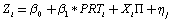
where Yi represents the fact that an individual has or not the particular kind of insurance under analysis, PRT stands for Proxy of Risk Tolerance, that is the behavioural variables discussed above, while Zi is the risk occurrence for the insurance studied, and Xi are the covariates (gender, age, education and marital status). We then run both the unconditional regression and the one controlled for the covariates. The control variables are used according to the usual insurance practices and are applied differently with respect to the insurance markets. Indeed, about the term life/long term insurance we will control for education, age and gender; then we will check the Medigap for education and age, the annuity for age, gender, education and marital status and the acute health only for education. We decided after careful consideration to use the probit in the model 1 because, although does not differ almost at all from a standard least squares regression model, it provides a better probabilistic interpretation. The model 2 is instead a classic least square estimation.
Since we should also embed somehow the differences due to being analysing different countries, we decide to follow the Bryan and Jenkins’ approach () on hierarchical (multilevel) datasets. According to them, to prove the robustness of our analysis we are going to run a simple pooled regression, a separate regression for each country and a country fixed effect model. This multiple choice could prove the results to be not related to the technique used and will improve the understanding of the phenomenon we are trying to capture providing different interpretations of the data.
First of all, a pooled regression with clustered-robust errors is going to be run. This would ignore that different countries have different unobserved features and will underestimate the standard errors of β, but it could be easily corrected using countries-robust standard errors that allow for a more general correlation within countries.
The second analysis implemented concerns instead a separate regression for each country. The country effect is in this way internalised and it is merged with the intercept of each regression model. It is a bit computationally more demanding, but it allows to put no restrictions on the variances of country-specific errors and to let β to vary across countries.
The final approach used is the fixed effect estimation, and it is set as a middle way between the two models explained above. It indeed pooled all the data but allows the intercept to differ across countries to be able to capture individual-specific effects. The other greatest difference with the single-country regression is that the residuals are here constrained to be the same across countries. Besides, it is useless to include further country-level variables, since the intercept embeds country differences. Every regression will then be corrected for cluster-robust errors and cross-sectionally weighted by the weights system provided by SHARE.
3 Results
The first two regressions presented in the Appendix are the pooled regressions. At a first glance, it seems that at an aggregate level the effects are not so weak, although very sparse. Indeed, as shown in Table 1, even if some of the results are generally either not significant or confirming the classic adverse selection theory, some relationships between insurance coverage and risky behaviours proved to be robust, meaningful and able to confirm our initial hypothesis of advantageous selection in European markets. Furthermore, the control variables seem to not affect considerably the estimation results. For instance, according to the classic theory individuals who currently smoke or drink should buy more insurance, but in reality they are more likely to buy less insurance. This is particularly true for long term care and term life/acute health respectively for smoking and drinking, and the same it is also verified for annuity markets and long term care for people physically inactive and for who implements more preventive health care actions. In addition, people not in the normality weight range are actually going to buy few insurance in three different markets, i.e. annuities, medigap and acute health.
Table 1
Relation between Insurance and Risky behaviours (Pooled Probit regression).
| Term life | Annuity | Lt care | Medigap | Acute health | ||||||
|---|---|---|---|---|---|---|---|---|---|---|
| No | Yes | No | Yes | No | Yes | No | Yes | No | Yes | |
| Main Smoking | 0.110* | 0.130** | 0.0389 | 0.0276 | –0.296*** | –0.277*** | –0.103 | –0.138 | –0.0322 | –0.0308 |
| (2.37) | (3.25) | (0.37) | (0.29) | (–5.43) | (–4.25) | (–1.08) | (–1.94) | (–0.49) | (–0.65) | |
| Drinking | –0.285*** | –0.310*** | –0.0729 | –0.0678 | –0.175 | –0.286 | 0.241 | 0.243 | –0.387*** | –0.389** |
| (–4.25) | (–5.28) | (–0.68) | (–0.66) | (–1.15) | (–1.88) | (1.43) | (1.87) | (–3.44) | (–3.26) | |
| BMI | 0.0283 | 0.0122 | –0.115** | –0.116 | –0.0138 | –0.114 | –0.151*** | –0.154*** | –0.311*** | –0.311*** |
| (0.59) | (0.23) | (–2.62) | (–1.91) | (–0.16) | (–1.70) | (–4.28) | (–3.33) | (–4.40) | (–4.70) | |
| Preventive | –0.0431 | –0.0363 | –0.100** | –0.110*** | 0.139 | 0.183 | –0.0598 | –0.0525 | 0.189** | 0.189** |
| (–1.17) | (–1.06) | (–3.25) | (–4.47) | (1.52) | (1.53) | (–1.37) | (–1.29) | (3.03) | (2.75) | |
| Inactivity | –0.179 | –0.215 | –0.408*** | –0.468*** | –0.716* | –0.819** | –0.146 | –0.0985 | –0.0624 | –0.0683 |
| (–0.97) | (–1.50) | (–7.19) | (–6.72) | (–2.13) | (–3.07) | (–1.49) | (–1.73) | (–0.62) | (–0.36) | |
| N | 2657 | 2657 | 22221 | 22221 | 1269 | 1269 | 22233 | 22233 | 1269 | 1269 |
There are two different regressions for each variable: on the left the unconstrained one, while on the right the one controlled for covariates.
*p < 0.05, **p < 0.01, ***p < 0.001.
In addition, the Table 2 shows that both smoking and physical inactivity increase the likely to die (and to not live long). While drinking seems to not be statistically significant in any circumstances, physical inactivity will also involve a higher level of medigap expenses as well as a higher likely to be hospitalised, as expected. On the other hand, preventive health actions reduce this risk and the smoking does not increase the chance to get hospitalised. This may seem counterintuitive, but since we considered a short time hospitalisation period and since the smoking effect are quite long term, it may be reasonable that the two variables are not positively correlated. Surprisingly, some anomalies characterise the BMI variable, meaning that the BMI seems to not reduce the life expectation. Further studies may be necessary in order to understand the reason why these kind of anomalies happen, but in general we may think of some psychological disease, misperception of the illness or simply the stress as possible causes of those strange phenomena, since it seems reasonable that people who, for example, are hypochondriac (or that somatizing a lot) are the ones who implement more prevention, who then spend more in extra medicines and cure and the ones who go to the hospital more likely as well. One general interpretation of the deviations presented is that maybe more risk averse individuals have less risky behaviours, and are the ones who value the insurance the most.
Table 2
Relation between Risk occurrence and Risky behaviours (Pooled LPM regression).
| Dead | Alive | Nursing Home | Medigap Exp | Hospital | ||||||
|---|---|---|---|---|---|---|---|---|---|---|
| No | Yes | No | Yes | No | Yes | No | Yes | No | Yes | |
| Smoking | –0.00399 | 0.00529* | –0.0217 | –0.0285 | –0.00198 | –0.000663 | –56.18 | –8.348 | –0.0223** | –0.0238*** |
| (–1.86) | (2.47) | (–1.33) | (–1.84) | (–1.42) | (–0.42) | (–1.20) | (–0.31) | (–3.92) | (–4.64) | |
| Drinking | 0.00745 | 0.0000605 | 0.0507 | 0.0483 | –0.00166 | –0.00272 | –45.09 | –42.96 | –0.00409 | –0.00232 |
| (1.87) | (0.01) | (1.87) | (1.93) | (–1.05) | (–1.23) | (–1.66) | (–1.28) | (–0.60) | (–0.29) | |
| BMI | –0.00285 | –0.00398 | 0.0202** | 0.0161** | –0.000794 | –0.000787 | –77.96 | –71.38 | 0.00773 | 0.00825 |
| (–0.88) | (–1.00) | (3.88) | (3.17) | (–0.42) | (–0.44) | (–0.96) | (–0.88) | (0.84) | (0.89) | |
| Preventive | 0.00267 | 0.00301 | –0.000823 | 0.00228 | –0.000145 | –0.000224 | –6.056 | –16.64 | 0.0262*** | 0.0260*** |
| (0.72) | (1.20) | (–0.11) | (0.29) | (–0.10) | (–0.16) | (–0.39) | (–1.08) | (9.14) | (8.91) | |
| Inactivity | 0.0777*** | 0.0635*** | –0.103* | –0.0841* | 0.0164 | 0.0151 | 253.3** | 190.1** | 0.169*** | 0.173*** |
| (12.06) | (10.11) | (–3.08) | (–2.68) | (1.81) | (1.90) | (4.05) | (3.93) | (17.17) | (13.96) | |
| N | 22233 | 22233 | 22233 | 22233 | 15040 | 15040 | 22233 | 22233 | 22226 | 22226 |
There are two different regressions for each variable: on the left the unconstrained one, while on the right the one controlled for covariates.
*p < 0.05, **p < 0.01, ***p < 0.001.
As above mentioned, the results are not verified for all the insurance markets and with respect to each dependent variable, but already in the comprehensive overall regression they provide robust insights about the advantageous selection issue.
After that, we run instead the Linear Probability Model analysis at a country-level. A regression for each country has been run and the results are visualised in Appendix as Figures 6, 7, 8, 9. There are five subgraphs corresponding to each insurance market and each coefficient for every independent variable is drawn by a smaller circle and a line that represents the confidence interval for that coefficient estimates at a level of 95%. For the sake of completeness, even if the results are not extremely different, the following figures have also the coefficient estimates taking into account the control variables. The results are clearly not so distant from the ones observed at an aggregate level, but they are again really mixed within each country and insurance market. What it should be noticed from these graphs are the numbers of point under/above the zero line, since as before we are more interested in the sign of the relations more than in the magnitude. In particular for the term life, the annuity and the medigap insurance markets, having riskier behaviours or taking less care about own health does not directly entail a higher demand of insurance. Again, the relation between the risk occurrence and the risky behaviours is instead generally confirmed, in particular regarding physical inactivity or the smoking addiction.
Relation between Insurance and Risky behaviours (LPM regression) per country.
Relation between Risk occurrence and Risky behaviours (LPM regression) per country.
Relation between Insurance and Risky behaviours (LPM regression) per country with control variables.
Relation between Risk occurrence and Risky behaviours (LPM regression) per country with control variables.
The final regressions showed in the Appendix regards the country fixed effect model (with cluster-robust errors), that is usually used in this situation because, with respect to for instance a random effect model, it underlines the unique features of each country. In the regressions run here, the control variables looked still to not have a crucial role.
The Table 3 points out again that, as expected, people who smoke or drink/with weight problems, are more likely to buy a term life or a long term care insurance, respectively. The opposite is instead verified still for smoking, drinking and BMI with respect to long term care, term life and acute health markets. The prevention is still ambiguous, since if from one hand shows an expected result such as the negative correlation with the annuity insurance purchase, on the other hand involves a positive relation with the acute health market, that is to some extent counterintuitive. Finally, physical inactivity proved again to provide the most robust results, i.e. it is negatively correlated with annuities, long term care and medigap as well. All our consideration may still make sense, behaviourally speaking, if we think again about people affected by apprehension or hypochondria, or physical inactivity reflected also in disregarding for personal care.
Table 3
Relation between Insurance and Risky behaviours with fixed-effect (Probit regression).
| Term life | Annuity | Lt care | Medigap | Acute health | ||||||
|---|---|---|---|---|---|---|---|---|---|---|
| No | Yes | No | Yes | No | Yes | No | Yes | No | Yes | |
| Main Smoking | 0.0947* | 0.120** | –0.00152 | 0.0190 | –0.347*** | –0.315*** | 0.0218 | –0.0340 | 0.0961 | 0.0445 |
| (2.40) | (2.70) | (–0.01) | (0.18) | (–5.78) | (–3.99) | (0.86) | (–1.68) | (1.29) | (0.70) | |
| Drinking | –0.194 | –0.227* | 0.161 | 0.0964 | 0.0955* | –0.0229 | 0.0988* | 0.0764 | –0.0981 | –0.0613 |
| (–1.76) | (–2.22) | (1.68) | (0.98) | (2.23) | (–0.33) | (2.00) | (1.74) | (–0.68) | (–0.37) | |
| BMI | 0.0435 | 0.0270 | –0.123 | –0.128 | 0.0999* | –0.00520 | –0.0804 | –0.0709 | –0.459*** | –0.464*** |
| (0.83) | (0.50) | (–1.90) | (–1.87) | (2.48) | (–0.12) | (–1.81) | (–1.49) | (–13.05) | (–14.13) | |
| Preventive | –0.0428 | –0.0376 | –0.111** | –0.104*** | 0.0757 | 0.102 | 0.0229 | 0.0337 | 0.150*** | 0.138** |
| (–1.18) | (–1.31) | (–3.10) | (–3.59) | (1.33) | (1.38) | (0.87) | (1.75) | (3.38) | (2.96) | |
| Inactivity | –0.193 | –0.241 | –0.290*** | –0.426*** | –0.835** | –0.890** | –0.234*** | –0.140* | 0.113 | 0.333*** |
| (–1.03) | (–1.58) | (–4.98) | (–5.02) | (–2.65) | (–3.12) | (–4.49) | (–2.38) | (0.79) | (3.53) | |
| N | 2657 | 2657 | 22221 | 22221 | 332 | 332 | 22233 | 22233 | 390 | 390 |
There are two different regressions for each variable: on the left the unconstrained one, while on the right the one controlled for covariates.
*p < 0.05, **p < 0.01, ***p < 0.001.
On the risk occurrence side instead (see Table 4), smoking is as expected associated to a higher chance to die (and to not live long), as well as physical inactivity, that proved also to be positively correlated with medigap expenses and hospitalisation. Prevention may require, as above mentioned, a higher possibility to get hospitalised, while counterintuitively the BMI is positively correlated with a higher life expectation and the smokers are less likely to go to the hospital (in one year time).
Table 4
Relation between Risk occurrence and Risky behaviours with fixed-effect (LPM regression).
| Dead | Alive | Nursing Home | Medigap Exp | Hospital | ||||||
|---|---|---|---|---|---|---|---|---|---|---|
| No | Yes | No | Yes | No | Yes | No | Yes | No | Yes | |
| Smoking | –0.00379 | 0.00536* | –0.0232 | –0.0344* | –0.00285* | –0.00141 | –67.52 | –20.02 | –0.0205** | –0.0200** |
| (–1.75) | (2.65) | (–1.60) | (–2.33) | (–2.76) | (–1.21) | (–1.66) | (–0.72) | (–4.08) | (–4.18) | |
| Drinking | 0.00629 | –0.00132 | 0.0212 | 0.0279 | 0.000407 | –0.000893 | –70.66 | –76.88 | 0.00319 | 0.00362 |
| (1.29) | (–0.25) | (1.31) | (1.46) | (0.31) | (–0.48) | (–1.28) | (–1.32) | (0.31) | (0.36) | |
| BMI | –0.00290 | –0.00383 | 0.0248*** | 0.0235*** | –0.00106 | –0.00121 | –82.38 | –71.16 | 0.00858 | 0.00831 |
| (–0.84) | (–0.95) | (8.55) | (6.04) | (–0.57) | (–0.70) | (–1.01) | (–0.91) | (1.05) | (0.97) | |
| Preventive | 0.00268 | 0.00300 | 0.00378 | 0.00498 | –0.000324 | –0.000322 | –4.803 | –15.51 | 0.0248*** | 0.0247*** |
| (0.74) | (1.21) | (0.42) | (0.65) | (–0.21) | (–0.23) | (–0.38) | (–1.11) | (9.41) | (9.56) | |
| Inactivity | 0.0780*** | 0.0639*** | –0.107*** | –0.0757** | 0.0183 | 0.0164 | 201.2* | 141.7 | 0.173*** | 0.172*** |
| (11.91) | (9.88) | (–5.18) | (–3.37) | (1.97) | (2.06) | (3.03) | (2.12) | (13.38) | (12.98) | |
| N | 22233 | 22233 | 22233 | 22233 | 15040 | 15040 | 22233 | 22233 | 22226 | 22226 |
There are two different regressions for each variable: on the left the unconstrained one, while on the right the one controlled for covariates.
*p < 0.05, **p < 0.01, ***p < 0.001.
Even in the country-fixed effect framework, although the results are less strong than in the pooled regression case, some anomaly seems to persist, and we believe the reasons behind this deviation could be interesting to be investigated in future works. We cannot conclude univocally in favour of our initial hypothesis neither in the fixed-effect scenario, but we can claim that the standard adverse selection theory seems to not hold strongly as the theory stated.
4 Conclusions
Our analysis aimed to investigate whether an advantageous selection phenomenon was proved to be robust in different insurance markets, as in Cutler et al. (). We focused on five insurance markets for eleven European countries plus Israel, specifically on term life, annuity, long term care, Medigap and acute health insurances. Our main finding has been that it looks like that riskier behaviours are not always associated with higher mortality, but above all they are not unconditionally associated with higher insurance demand as the classic theory would predict. This result does not hold for each country and each market with respect to each risky behaviour, but the outcomes are mixed, suggesting that further analysis may shine a light on this puzzle. In particular, in the most robust analysis, no systematic relation between risky behaviours and any of the insurance market, although some risky behaviours are not coherent (while others are) with Rothschild and Stiglitz (). In any case, it is interesting to notice that the adverse selection proposed in the ‘70s does not hold anymore so strongly and extensively, but also to consider that maybe preferences heterogeneity for insurance could explain the different behaviours of the participants. A different risk tolerance may indeed explain the insurance puzzle, but of course further investigations will be required in order to test this hypothesis.